AP® Calculus AB Cheat Sheet

Last Updated: September 23, 2024

Notes

This AP Calculus AB Cheat Sheet provides a concise overview of essential formulas, key concepts, and critical information from the AP Calculus AB curriculum. Covering all major topics, it simplifies complex ideas into easy-to-understand points, helping students quickly review and solidify their understanding. With important calculus formulas, theorems, and example problems, students can effectively apply these concepts to both multiple-choice and free-response questions. Organized into clear sections with step-by-step explanations, this cheat sheet is a valuable tool for mastering the exam and achieving top scores in AP Calculus AB.

Free AP Calculus AB Practice Test

Download AP Calculus AB Cheatsheet – Pdf

Unit 1: Limits & Continuity

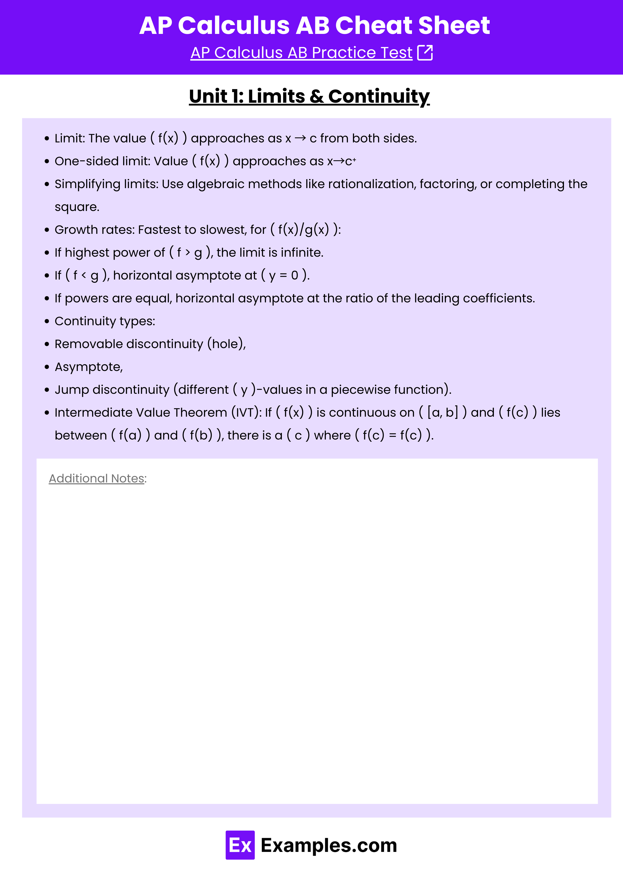
Limit: The value ( f(x) ) approaches as x → c from both sides.
One-sided limit: Value ( f(x) ) approaches as x→c⁺
Simplifying limits: Use algebraic methods like rationalization, factoring, or completing the square.
Growth rates: Fastest to slowest, for ( f(x)/g(x) ):
If highest power of ( f > g ), the limit is infinite.
If ( f < g ), horizontal asymptote at ( y = 0 ).
If powers are equal, horizontal asymptote at the ratio of the leading coefficients.
Continuity types:
Removable discontinuity (hole),
Asymptote,
Jump discontinuity (different ( y )-values in a piecewise function).
Intermediate Value Theorem (IVT): If ( f(x) ) is continuous on ( [a, b] ) and ( f(c) ) lies between ( f(a) ) and ( f(b) ), there is a ( c ) where ( f(c) = f(c) ).

Unit 2: Differentiation: Definition and Fundamental Properties

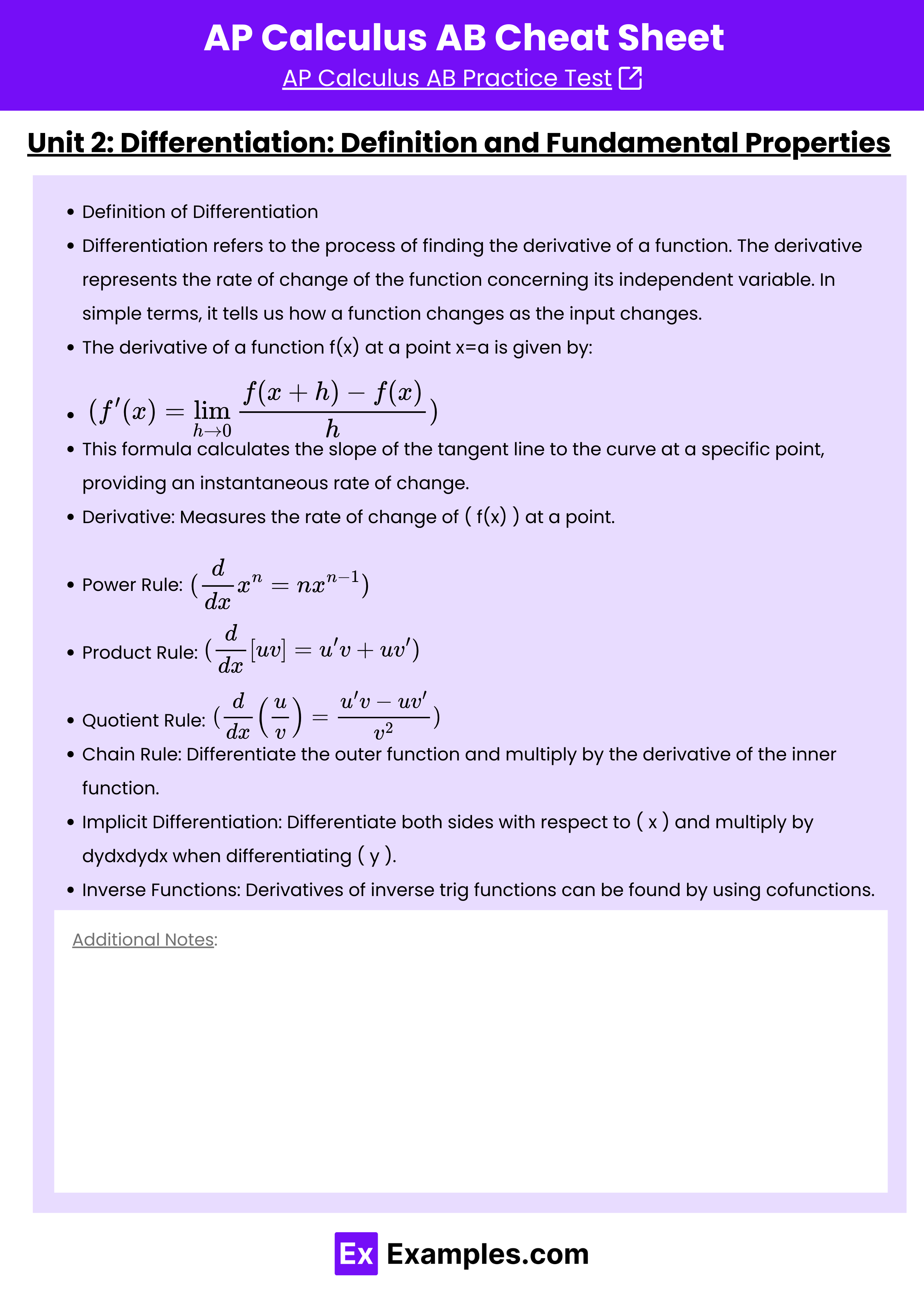
Definition of Differentiation

Differentiation refers to the process of finding the derivative of a function. The derivative represents the rate of change of the function concerning its independent variable. In simple terms, it tells us how a function changes as the input changes.

The derivative of a function f(x) at a point x=a is given by:

$f'(x) = \lim_{h \to 0} \frac{f(x + h) - f(x)}{h}$

This formula calculates the slope of the tangent line to the curve at a specific point, providing an instantaneous rate of change.

Derivative: Measures the rate of change of ( f(x) ) at a point.
Power Rule: $\frac{d}{dx} x^n = n x^{n-1}$
Product Rule: $\frac{d}{dx} [uv] = u'v + uv'$
Quotient Rule: $\frac{d}{dx} \left( \frac{u}{v} \right) = \frac{u'v - uv'}{v^2}$
Chain Rule: Differentiate the outer function and multiply by the derivative of the inner function.
Implicit Differentiation: Differentiate both sides with respect to ( x ) and multiply by $\frac{dy}{dx}$ when differentiating ( y ).
Inverse Functions: Derivatives of inverse trig functions can be found by using cofunctions.

Unit 3: Differentiation of Composite, Implicit, and Inverse Functions

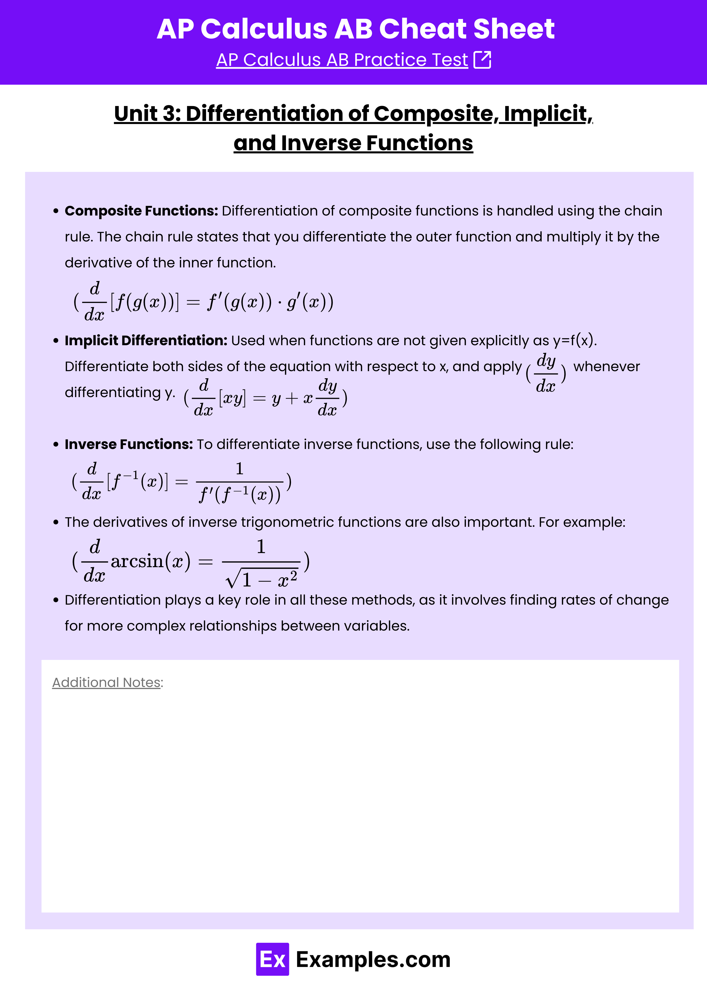
Composite Functions: Differentiation of composite functions is handled using the chain rule. The chain rule states that you differentiate the outer function and multiply it by the derivative of the inner function.

$\frac{d}{dx} [f(g(x))] = f'(g(x)) \cdot g'(x)$

Implicit Differentiation: Used when functions are not given explicitly as y=f(x). Differentiate both sides of the equation with respect to x, and apply $\frac{dy}{dx}$ whenever differentiating y.

$\frac{d}{dx} [xy] = y + x \frac{dy}{dx}$

Inverse Functions: To differentiate inverse functions, use the following rule:

$\frac{d}{dx} [f^{-1}(x)] = \frac{1}{f'(f^{-1}(x))}$

The derivatives of inverse trigonometric functions are also important. For example:

$\frac{d}{dx} \arcsin(x) = \frac{1}{\sqrt{1 - x^2}}$

Differentiation plays a key role in all these methods, as it involves finding rates of change for more complex relationships between variables.

Unit 4: Contextual Applications of Differentiation

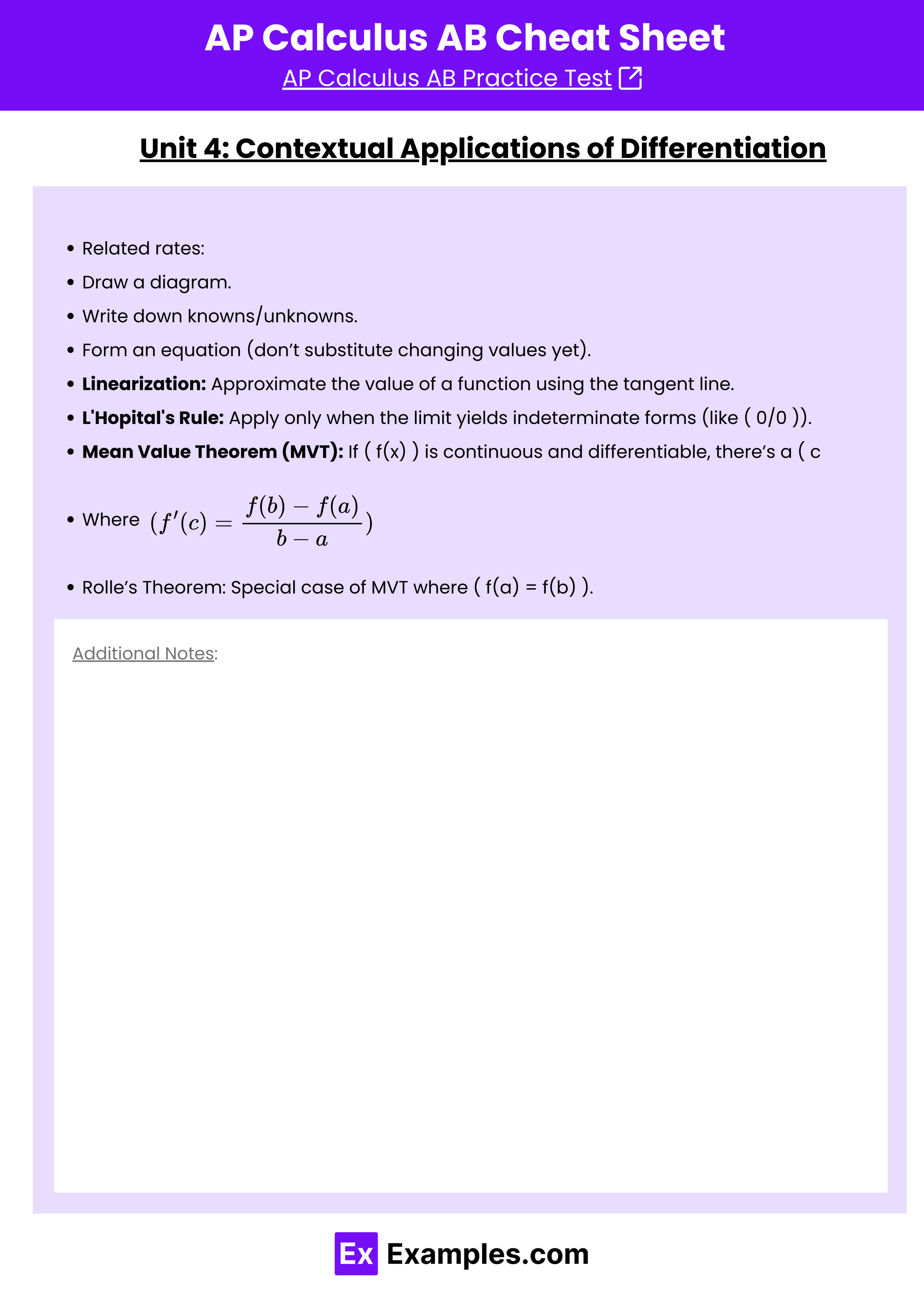
Related rates:

Draw a diagram.
Write down knowns/unknowns.
Form an equation (don’t substitute changing values yet).

Linearization: Approximate the value of a function using the tangent line.
L’Hopital’s Rule: Apply only when the limit yields indeterminate forms (like ( 0/0 )).
Mean Value Theorem (MVT): If ( f(x) ) is continuous and differentiable, there’s a ( c ) Where $f'(c) = \frac{f(b) - f(a)}{b - a}$
Rolle’s Theorem: Special case of MVT where ( f(a) = f(b) ).

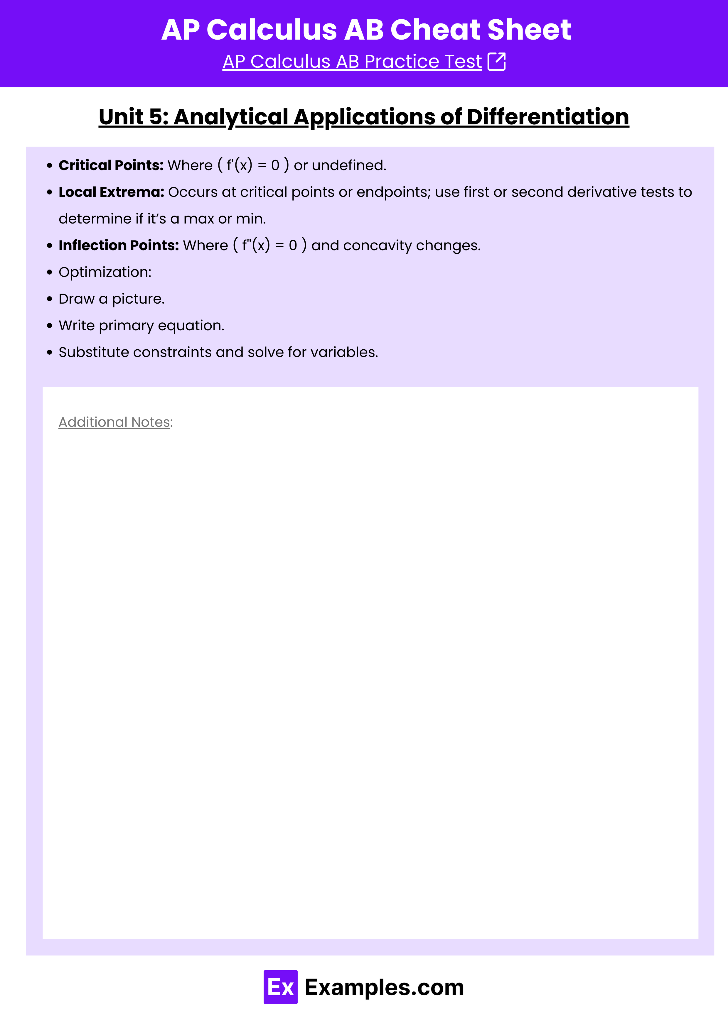
Unit 5: Analytical Applications of Differentiation

Critical Points: Where ( f'(x) = 0 ) or undefined.
Local Extrema: Occurs at critical points or endpoints; use first or second derivative tests to determine if it’s a max or min.
Inflection Points: Where ( f”(x) = 0 ) and concavity changes.
Optimization:

Draw a picture.
Write primary equation.
Substitute constraints and solve for variables.

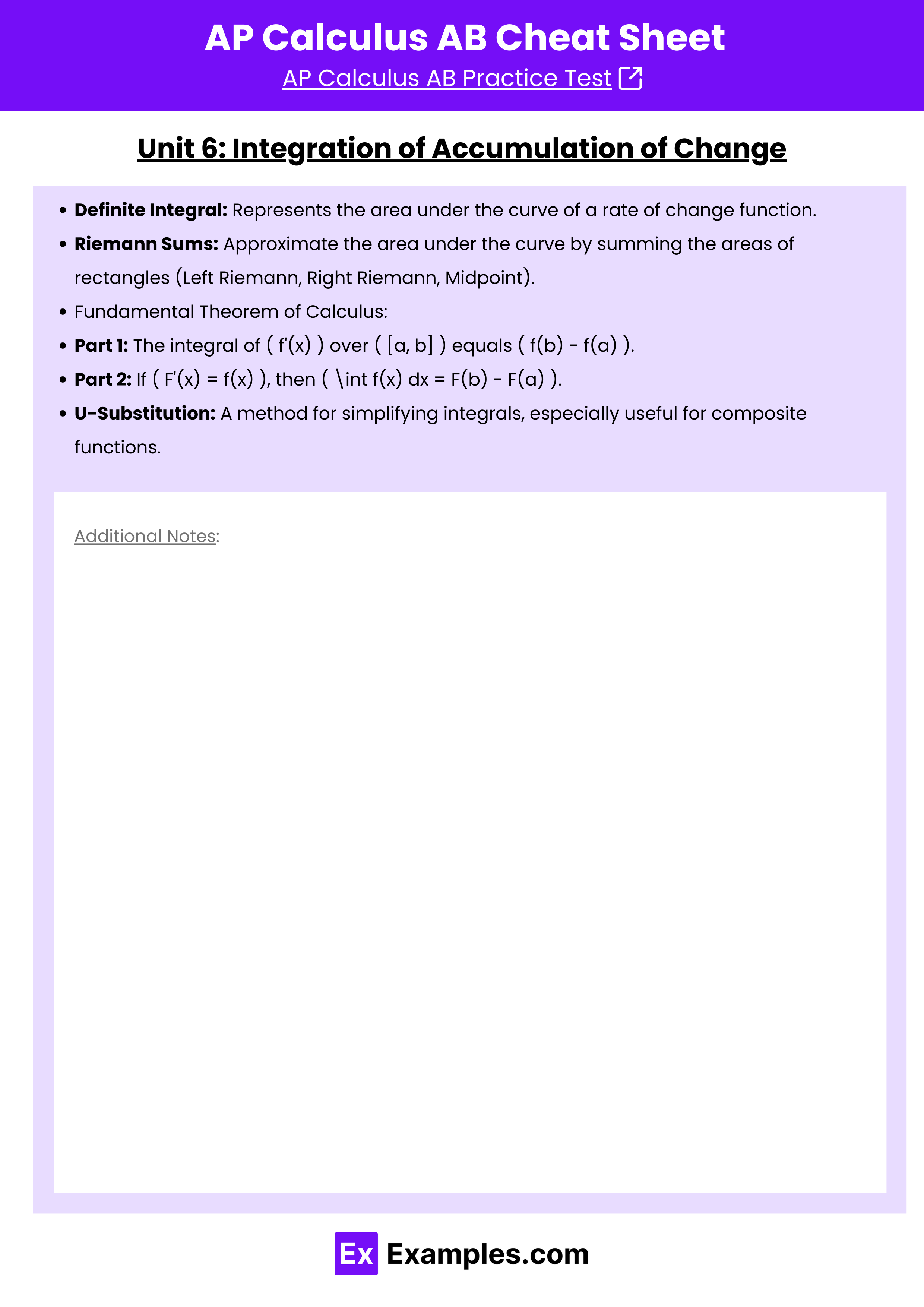
Unit 6: Integration of Accumulation of Change

Definite Integral: Represents the area under the curve of a rate of change function.
Riemann Sums: Approximate the area under the curve by summing the areas of rectangles (Left Riemann, Right Riemann, Midpoint).
Fundamental Theorem of Calculus:
Part 1: The integral of ( f'(x) ) over ( [a, b] ) equals ( f(b) – f(a) ).
Part 2: If ( F'(x) = f(x) ), then ( \int f(x) dx = F(b) – F(a) ).
U-Substitution: A method for simplifying integrals, especially useful for composite functions.

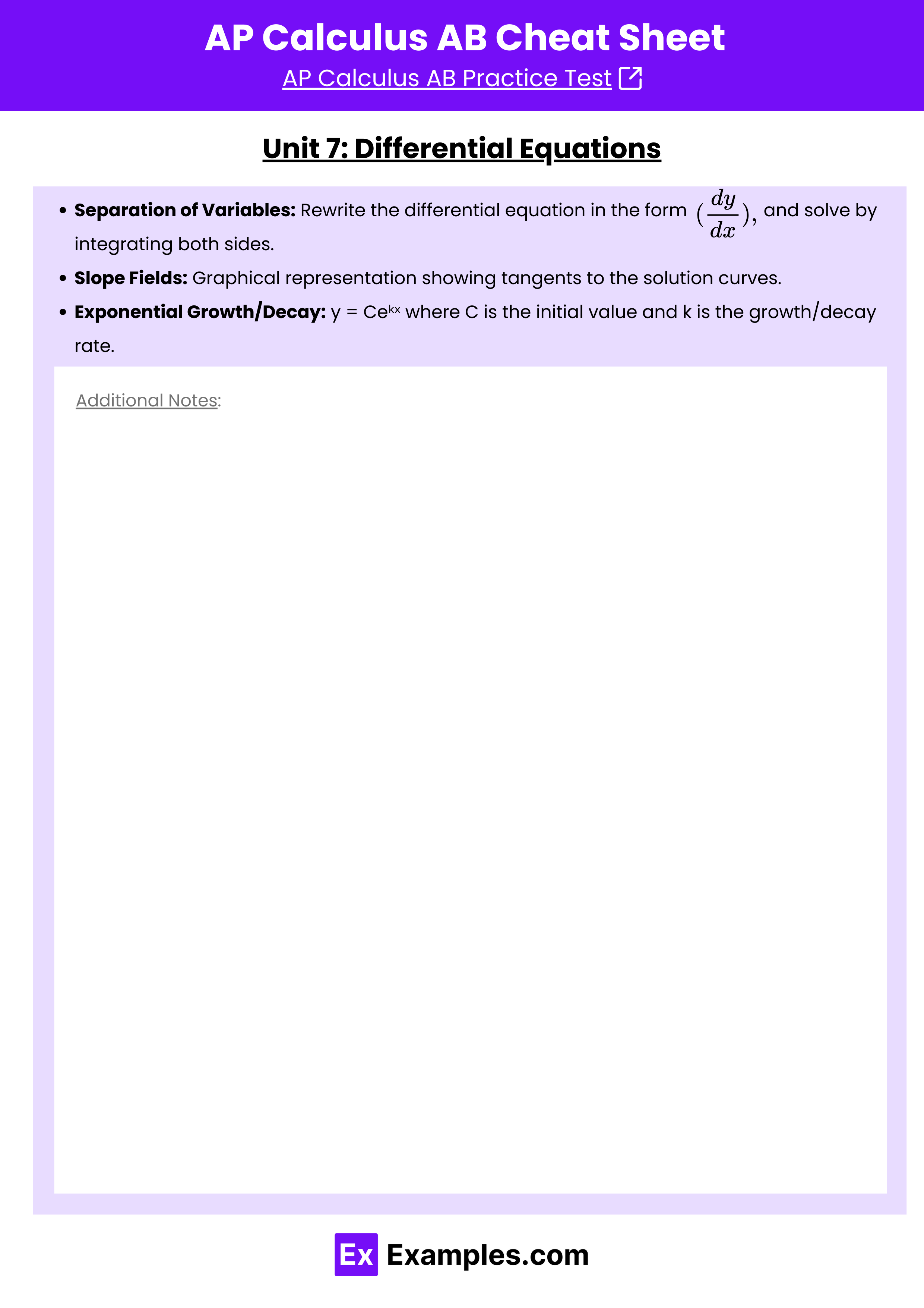
Unit 7: Differential Equations

Separation of Variables: Rewrite the differential equation in the form $\frac{dy}{dx}$ , and solve by integrating both sides.
Slope Fields: Graphical representation showing tangents to the solution curves.
Exponential Growth/Decay: y = Ceᵏˣ where C is the initial value and k is the growth/decay rate.

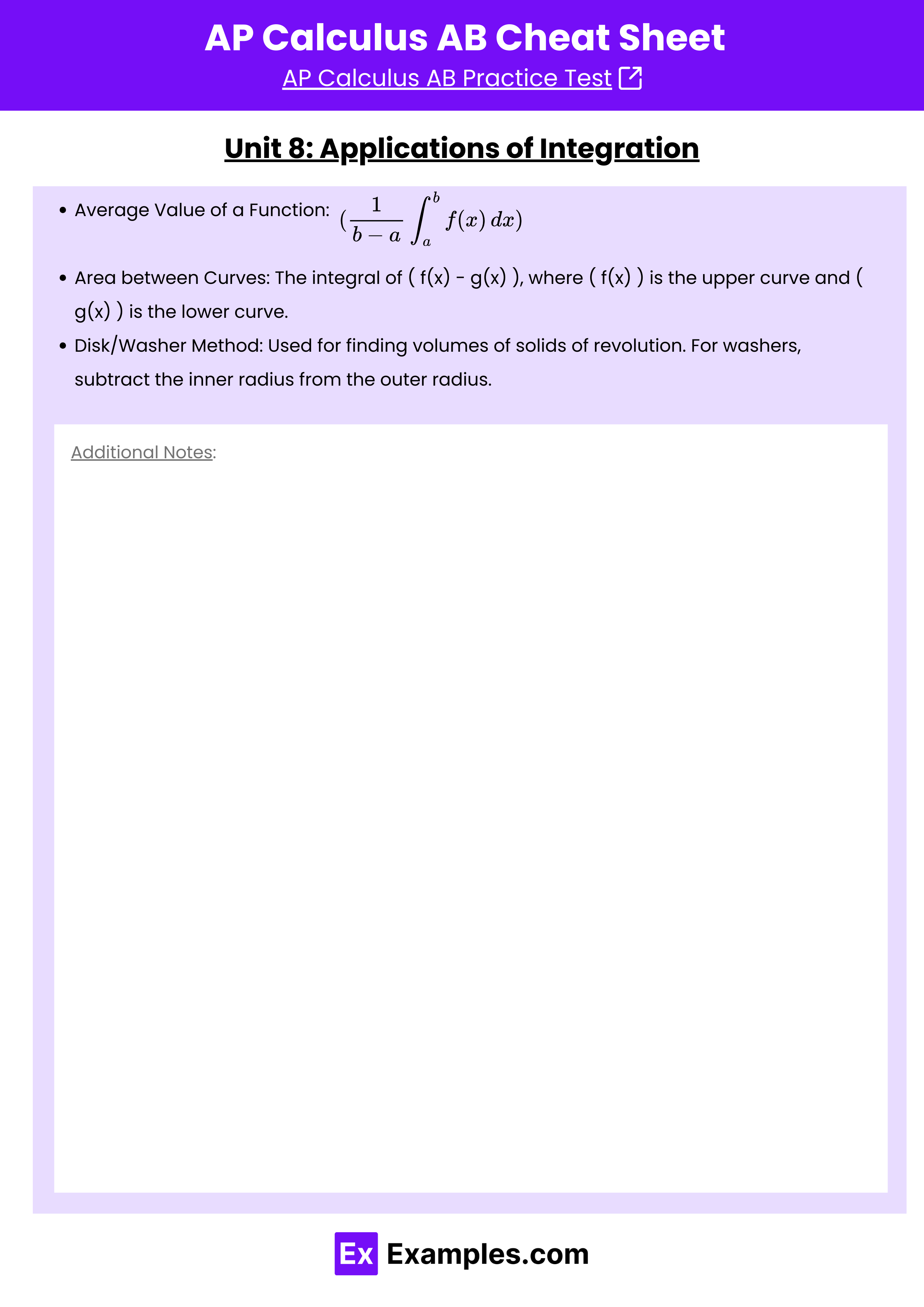
Unit 8: Applications of Integration

Average Value of a Function: $\frac{1}{b - a} \int_{a}^{b} f(x)\, dx$
Area between Curves: The integral of ( f(x) – g(x) ), where ( f(x) ) is the upper curve and ( g(x) ) is the lower curve.
Disk/Washer Method: Used for finding volumes of solids of revolution. For washers, subtract the inner radius from the outer radius.