

Snowflake for Developers
/
Guides
QUICKSTART
Zero to Snowflake
Dynamic Tables
Cameron Shimmin, Dureti Shemsi
FORK REPO
Overview
Overview
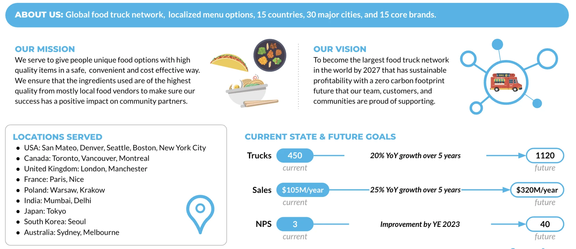
Who is Tasty Bytes?
Welcome to the Zero to Snowflake Quickstart! This guide is a consolidated journey through key areas of the Snowflake AI Data Cloud. You will start
with the fundamentals of warehousing and data transformation, build an automated data pipeline, then see how you can experiment with LLMs
using the Cortex Playground to compare different models for summarizing text, use AISQL Functions to instantly analyze customer review
sentiment with a simple SQL command, and harness Cortex Search for intelligent text discovery, and utilize Cortex Analyst for conversational
business intelligence. Finally, you will learn to secure your data with powerful governance controls and enrich your analysis through seamless data
collaboration.
We'll apply these concepts using a sample dataset from our fictitious food truck, Tasty Bytes, to improve and streamline their data operations. We'll
explore this dataset through several workload-specific scenarios, demonstrating the benefits Snowflake provides to businesses.
Expedition. Free, virtual, Nov 3–6.
Technical tracks for practitioners, outcomes for leaders.
Register now
9/26/26, 12:02 PM
Zero to Snowflake
https://www.snowflake.com/en/developers/guides/zero-to-snowflake/
1/59
Prerequisites
What You Will Learn
What You Will Build
Setup
Overview
Step 1 - Create Your Setup SQL File
Step 2 - Add and Run the Setup Script
Our mission is to provide unique, high-quality food options in a convenient and cost-effective manner, emphasizing the use of fresh ingredients
from local vendors. Their vision is to become the largest food truck network in the world with a zero carbon footprint.
A Supported Snowflake
Browser
An Enterprise or Business Critical Snowflake Account
If you do not have a Snowflake Account, please
sign up for a Free 30 Day Trial Account
. When signing up, please make sure to select Enterprise
edition. You are welcome to choose any
Snowflake Cloud/Region
.
After registering, you will receive an email with an activation link and your Snowflake Account URL.
Vignette 1: Getting Started with Snowflake:
The fundamentals of Snowflake warehouses, caching, cloning, and Time Travel.
Vignette 2: Simple Data Pipelines:
How to ingest and transform semi-structured data using Dynamic Tables.
Vignette 3: Snowflake Cortex AI:
How to leverage Snowflake's comprehensive AI capabilities for experimentation, scalable analysis, AI-assisted
development, and conversational business intelligence.
Vignette 4: Governance with Horizon:
How to protect your data with roles, classification, masking, and row-access policies.
Vignette 5: Apps & Collaboration:
How to leverage the Snowflake Marketplace to enrich your internal data with third-party datasets.
A comprehensive understanding of the core Snowflake platform.
Configured Virtual Warehouses.
An automated ELT pipeline with Dynamic Tables.
A complete intelligence customer analytics platform leveraging Snowflake AI.
A robust data governance framework with roles and policies.
Enriched analytical views combining first- and third-party data.
In this guide, we will use
Snowflake Workspaces
to organize, edit, and run all the SQL scripts required for this course. We will create a dedicated
SQL file for the setup and each vignette. This will keep our code organized and easy to manage.
Let's walk through how to create your first SQL file, add the necessary setup code, and run it.
First, we need a place to put our setup script.
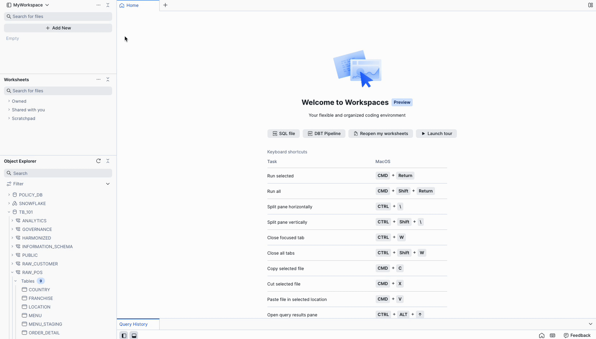
1.
Navigate to
Workspaces
:
In the left-hand navigation menu of the Snowflake UI, click on
Projects
»
Workspaces
. This is the central hub for all
your SQL files.
2.
Create a New SQL File:
Find and click the
+ Add New
button in the top-left corner of the
Workspaces
area, then select
SQL File
. This will
generate a new, blank SQL file.
3.
Rename the SQL File:
Your new SQL file will have a name based on the timestamp it was created. Give it a descriptive name like
Zero To
Snowflake - Setup
.
Now that you have your SQL file, it's time to add the setup SQL and execute it.
1.
Copy the SQL Code:
Click the link for the
setup file
and copy it to your clipboard.
2.
Paste into your SQL File:
Return to your Zero To Snowflake Setup SQL file in Snowflake and paste the entire script into the editor.
START FOR FREE
9/26/26, 12:02 PM
Zero to Snowflake
https://www.snowflake.com/en/developers/guides/zero-to-snowflake/
2/59

Looking Ahead
Get Started with Snowflake
Overview
What You Will Learn
3.
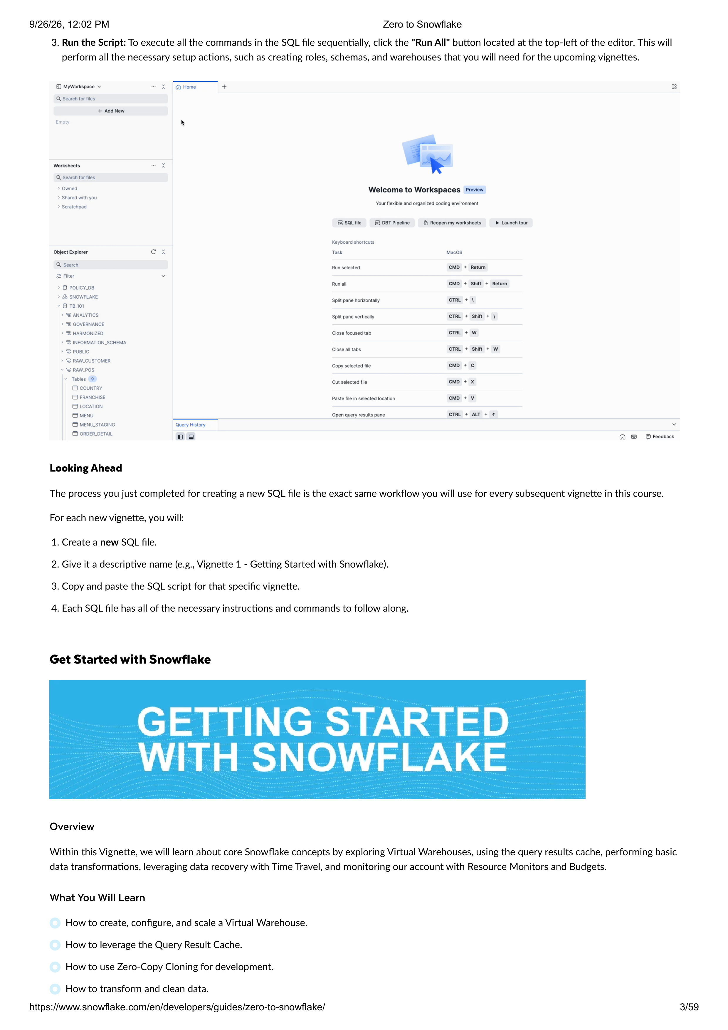
Run the Script:
To execute all the commands in the SQL file sequentially, click the
"Run All"
button located at the top-left of the editor. This will
perform all the necessary setup actions, such as creating roles, schemas, and warehouses that you will need for the upcoming vignettes.
The process you just completed for creating a new SQL file is the exact same workflow you will use for every subsequent vignette in this course.
For each new vignette, you will:
1. Create a
new
SQL file.
2. Give it a descriptive name (e.g., Vignette 1 - Getting Started with Snowflake).
3. Copy and paste the SQL script for that specific vignette.
4. Each SQL file has all of the necessary instructions and commands to follow along.
Within this Vignette, we will learn about core Snowflake concepts by exploring Virtual Warehouses, using the query results cache, performing basic
data transformations, leveraging data recovery with Time Travel, and monitoring our account with Resource Monitors and Budgets.
How to create, configure, and scale a Virtual Warehouse.
How to leverage the Query Result Cache.
How to use Zero-Copy Cloning for development.
How to transform and clean data.
9/26/26, 12:02 PM
Zero to Snowflake
https://www.snowflake.com/en/developers/guides/zero-to-snowflake/
3/59
What You Will Build
Get the SQL code and paste it into your SQL File.
Virtual Warehouses and Settings
Overview
Step 1 - Setting Context
Step 2 - Creating a Warehouse
Step 3 - Using and Resuming a Warehouse
How to instantly recover a dropped table using UNDROP.
How to create and apply a Resource Monitor.
How to create a Budget to monitor costs.
How to use Universal Search to find objects and information.
A Snowflake Virtual Warehouse
A development copy of a table using Zero-Copy Clone
A Resource Monitor
A Budget
Copy and paste the SQL code from this
file
in a new SQL File to follow along in Snowflake. Note that once you've reached the end of the SQL File
you can skip to Step 10 - Simple Data Pipeline
Virtual Warehouses are the dynamic, scalable, and cost-effective computing power that lets you perform analysis on your Snowflake data. Their
purpose is to handle all your data processing needs without you having to worry about the underlying technical details.
First, lets set our session context. To run the queries, highlight the three queries at the top of your SQL file and click the "
►
Run" button.
ALTER SESSION SET query_tag = '{"origin":"sf_sit-is","name":"tb_zts,"version":{"major":1, "minor":1},"attribut
ALTER SESSION SET query_tag = '{"origin":"sf_sit-is","name":"tb_zts,"version":{"major":1, "minor":1},"attribut
USE DATABASE tb_101;
USE DATABASE tb_101;
USE ROLE accountadmin;
USE ROLE accountadmin;
Let's create our first warehouse! This command creates a new X-Small warehouse that will initially be suspended.
CREATE OR REPLACE WAREHOUSE my_wh
CREATE OR REPLACE WAREHOUSE my_wh
COMMENT = 'My TastyBytes warehouse'
COMMENT = 'My TastyBytes warehouse'
WAREHOUSE_TYPE = 'standard'
WAREHOUSE_TYPE = 'standard'
WAREHOUSE_SIZE = 'xsmall'
WAREHOUSE_SIZE = 'xsmall'
MIN_CLUSTER_COUNT = 1
MIN_CLUSTER_COUNT = 1
MAX_CLUSTER_COUNT = 2
MAX_CLUSTER_COUNT = 2
SCALING_POLICY = 'standard'
SCALING_POLICY = 'standard'
AUTO_SUSPEND = 60
AUTO_SUSPEND = 60
INITIALLY_SUSPENDED = true
INITIALLY_SUSPENDED = true
AUTO_RESUME = false;
AUTO_RESUME = false;
Virtual Warehouses
: A virtual warehouse, often referred to simply as a “warehouse”, is a cluster of compute resources in
Snowflake. Warehouses are required for queries, DML operations, and data loading. For more information, see the
Warehouse
Overview
.
Now that we have a warehouse, we must set it as the active warehouse for our session. Execute the next statement.
USE WAREHOUSE my_wh;
USE WAREHOUSE my_wh;
9/26/26, 12:02 PM
Zero to Snowflake
https://www.snowflake.com/en/developers/guides/zero-to-snowflake/
4/59

Step 4 - Scaling a Warehouse
Query Result Cache
Overview
Step 1 - Re-running a Query
If you try to run the query below, it will fail, because the warehouse is suspended and does not have
AUTO_RESUME
enabled.
SELECT * FROM raw_pos.truck_details;
SELECT * FROM raw_pos.truck_details;
Let's resume it and set it to auto-resume in the future.
ALTER WAREHOUSE my_wh RESUME;
ALTER WAREHOUSE my_wh RESUME;
ALTER WAREHOUSE my_wh SET AUTO_RESUME = TRUE;
ALTER WAREHOUSE my_wh SET AUTO_RESUME = TRUE;
Now, try the query again. It should execute successfully.
SELECT * FROM raw_pos.truck_details;
SELECT * FROM raw_pos.truck_details;
Warehouses in Snowflake are designed for elasticity. We can scale our warehouse up on the fly to handle a more intensive workload. Let's scale our
warehouse to an X-Large.
ALTER WAREHOUSE my_wh SET warehouse_size = 'XLarge';
ALTER WAREHOUSE my_wh SET warehouse_size = 'XLarge';
With our larger warehouse, let's run a query to calculate total sales per truck brand.
SELECT
SELECT
o.truck_brand_name,
o.truck_brand_name,
COUNT(DISTINCT o.order_id) AS order_count,
COUNT(DISTINCT o.order_id) AS order_count,
SUM(o.price) AS total_sales
SUM(o.price) AS total_sales
FROM analytics.orders_v o
FROM analytics.orders_v o
GROUP BY o.truck_brand_name
GROUP BY o.truck_brand_name
ORDER BY total_sales DESC;
ORDER BY total_sales DESC;
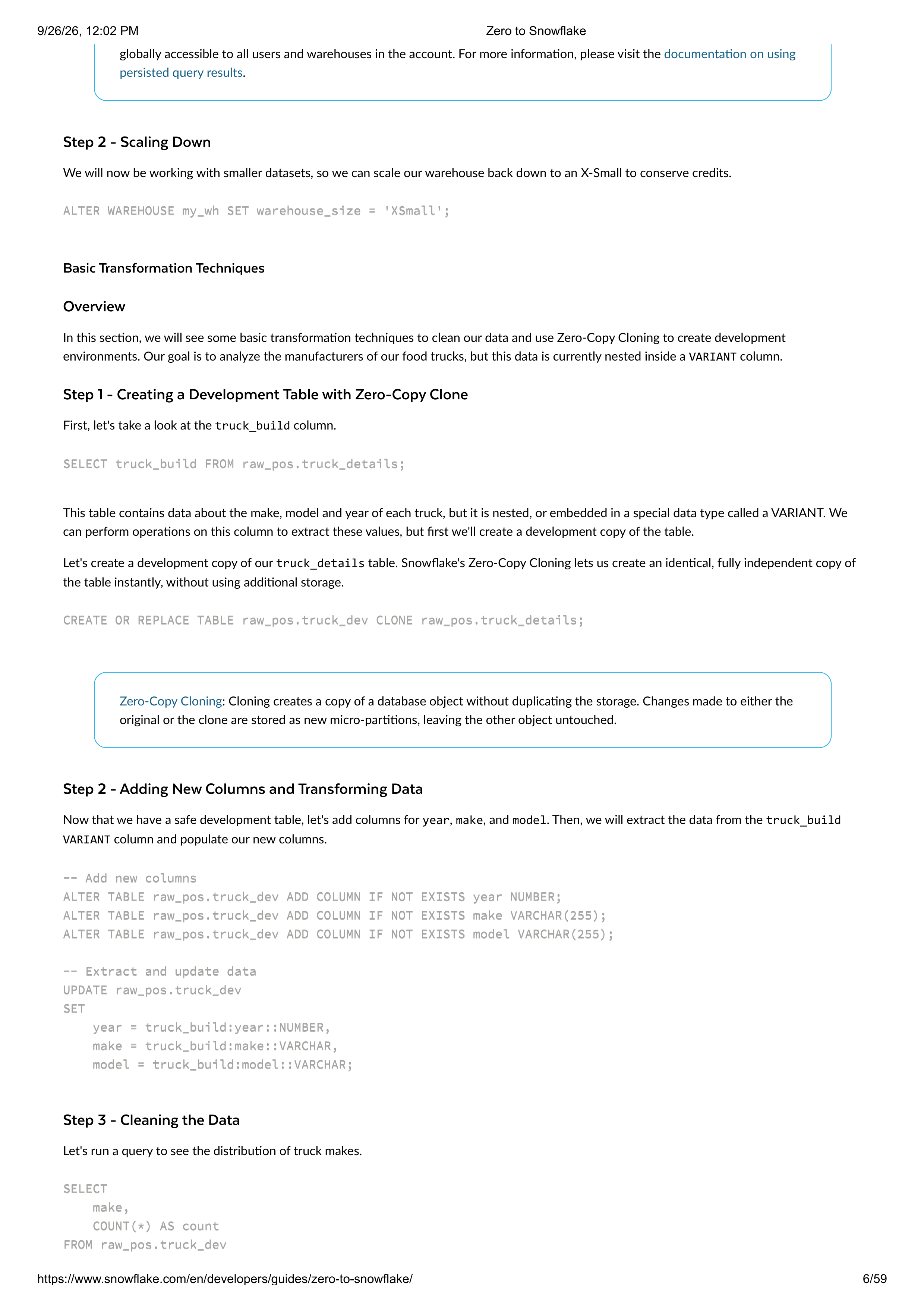
This is a great place to demonstrate another powerful feature in Snowflake: the Query Result Cache. When you first ran the 'sales per truck' query,
it likely took several seconds. If you run the exact same query again, the result will be nearly instantaneous. This is because the query results were
cached in Snowflake's Query Result Cache.
Run the same 'sales per truck' query from the previous step. Note the execution time in the query details pane. It should be much faster.
SELECT
SELECT
o.truck_brand_name,
o.truck_brand_name,
COUNT(DISTINCT o.order_id) AS order_count,
COUNT(DISTINCT o.order_id) AS order_count,
SUM(o.price) AS total_sales
SUM(o.price) AS total_sales
FROM analytics.orders_v o
FROM analytics.orders_v o
GROUP BY o.truck_brand_name
GROUP BY o.truck_brand_name
ORDER BY total_sales DESC;
ORDER BY total_sales DESC;
Query Result Cache
: Results are retained for any query for 24 hours. Hitting the result cache requires almost no compute
resources, making it ideal for frequently run reports or dashboards. The cache resides in the Cloud Services Layer, making it
9/26/26, 12:02 PM
Zero to Snowflake
https://www.snowflake.com/en/developers/guides/zero-to-snowflake/
5/59
Step 2 - Scaling Down
Basic Transformation Techniques
Overview
Step 1 - Creating a Development Table with Zero-Copy Clone
Step 2 - Adding New Columns and Transforming Data
Step 3 - Cleaning the Data
globally accessible to all users and warehouses in the account. For more information, please visit the
documentation on using
persisted query results
.
We will now be working with smaller datasets, so we can scale our warehouse back down to an X-Small to conserve credits.
ALTER WAREHOUSE my_wh SET warehouse_size = 'XSmall';
ALTER WAREHOUSE my_wh SET warehouse_size = 'XSmall';
In this section, we will see some basic transformation techniques to clean our data and use Zero-Copy Cloning to create development
environments. Our goal is to analyze the manufacturers of our food trucks, but this data is currently nested inside a
VARIANT
column.
First, let's take a look at the
truck_build
column.
SELECT truck_build FROM raw_pos.truck_details;
SELECT truck_build FROM raw_pos.truck_details;
This table contains data about the make, model and year of each truck, but it is nested, or embedded in a special data type called a VARIANT. We
can perform operations on this column to extract these values, but first we'll create a development copy of the table.
Let's create a development copy of our
truck_details
table. Snowflake's Zero-Copy Cloning lets us create an identical, fully independent copy of
the table instantly, without using additional storage.
CREATE OR REPLACE TABLE raw_pos.truck_dev CLONE raw_pos.truck_details;
CREATE OR REPLACE TABLE raw_pos.truck_dev CLONE raw_pos.truck_details;
Zero-Copy Cloning
: Cloning creates a copy of a database object without duplicating the storage. Changes made to either the
original or the clone are stored as new micro-partitions, leaving the other object untouched.
Now that we have a safe development table, let's add columns for
year
,
make
, and
model
. Then, we will extract the data from the
truck_build
VARIANT
column and populate our new columns.
-- Add new columns
-- Add new columns
ALTER TABLE raw_pos.truck_dev ADD COLUMN IF NOT EXISTS year NUMBER;
ALTER TABLE raw_pos.truck_dev ADD COLUMN IF NOT EXISTS year NUMBER;
ALTER TABLE raw_pos.truck_dev ADD COLUMN IF NOT EXISTS make VARCHAR(255);
ALTER TABLE raw_pos.truck_dev ADD COLUMN IF NOT EXISTS make VARCHAR(255);
ALTER TABLE raw_pos.truck_dev ADD COLUMN IF NOT EXISTS model VARCHAR(255);
ALTER TABLE raw_pos.truck_dev ADD COLUMN IF NOT EXISTS model VARCHAR(255);
-- Extract and update data
-- Extract and update data
UPDATE raw_pos.truck_dev
UPDATE raw_pos.truck_dev
SET
SET
year = truck_build:year::NUMBER,
year = truck_build:year::NUMBER,
make = truck_build:make::VARCHAR,
make = truck_build:make::VARCHAR,
model = truck_build:model::VARCHAR;
model = truck_build:model::VARCHAR;
Let's run a query to see the distribution of truck makes.
SELECT
SELECT
make,
make,
COUNT(*) AS count
COUNT(*) AS count
FROM raw_pos.truck_dev
FROM raw_pos.truck_dev
9/26/26, 12:02 PM
Zero to Snowflake
https://www.snowflake.com/en/developers/guides/zero-to-snowflake/
6/59
Step 4 - Promoting to Production with SWAP
Step 5 - Cleanup
Step 6 - Data Recovery with UNDROP
Step 7 - Verify the Drop
Step 8 - Restore the Table with UNDROP
Step 9 - Verify Restoration and Clean Up
GROUP BY make
GROUP BY make
ORDER BY make ASC;
ORDER BY make ASC;
Did you notice anything odd about the results from the last query? We can see a data quality issue: 'Ford' and 'Ford_' are being treated as separate
manufacturers. Let's easily fix this with a simple
UPDATE
statement.
UPDATE raw_pos.truck_dev
UPDATE raw_pos.truck_dev
SET make = 'Ford'
SET make = 'Ford'
WHERE make = 'Ford_';
WHERE make = 'Ford_';
Here we're saying we want to set the row's make value to
Ford
wherever it is
Ford_
. This will ensure none of the Ford makes have the underscore,
giving us a unified make count.
Our development table is now cleaned and correctly formatted. We can instantly promote it to be the new production table using the
SWAP WITH
command. This atomically swaps the two tables.
ALTER TABLE raw_pos.truck_details SWAP WITH raw_pos.truck_dev;
ALTER TABLE raw_pos.truck_details SWAP WITH raw_pos.truck_dev;
Now that the swap is complete, we can drop the unnecessary
truck_build
column from our new production table. We also need to drop the old
production table, which is now named
truck_dev
. But for the sake of the next lesson, we will "accidentally" drop the main table.
ALTER TABLE raw_pos.truck_details DROP COLUMN truck_build;
ALTER TABLE raw_pos.truck_details DROP COLUMN truck_build;
-- Accidentally drop the production table!
-- Accidentally drop the production table!
DROP TABLE raw_pos.truck_details;
DROP TABLE raw_pos.truck_details;
Oh no! We accidentally dropped the production
truck_details
table. Luckily, Snowflake's Time Travel feature allows us to recover it instantly. The
UNDROP
command restores dropped objects.
If you run a
DESCRIBE
command on the table, you will get an error stating it does not exist.
DESCRIBE TABLE raw_pos.truck_details;
DESCRIBE TABLE raw_pos.truck_details;
Let's restore the
truck_details
table to the exact state it was in before being dropped.
UNDROP TABLE raw_pos.truck_details;
UNDROP TABLE raw_pos.truck_details;
Time Travel & UNDROP
: Snowflake Time Travel enables accessing historical data at any point within a defined period. This
allows for restoring data that has been modified or deleted.
UNDROP
is a feature of Time Travel that makes recovery from
accidental drops trivial.
Verify the table was successfully restored by selecting from it. Then, we can safely drop the actual development table,
truck_dev
.
-- Verify the table was restored
-- Verify the table was restored
SELECT * from raw_pos.truck_details;
SELECT * from raw_pos.truck_details;
9/26/26, 12:02 PM
Zero to Snowflake
https://www.snowflake.com/en/developers/guides/zero-to-snowflake/
7/59
Resource Monitors
Overview
Step 1 - Creating a Resource Monitor
Step 2 - Applying the Resource Monitor
Create a Budget
Overview
Step 1 - Creating a Budget via SQL
Step 2 - Budget Page in Snowsight
-- Now drop the real truck_dev table
-- Now drop the real truck_dev table
DROP TABLE raw_pos.truck_dev;
DROP TABLE raw_pos.truck_dev;
Monitoring compute usage is critical. Snowflake provides Resource Monitors to track warehouse credit usage. You can define credit quotas and
trigger actions (like notifications or suspension) when thresholds are reached.
Let's create a resource monitor for
my_wh
. This monitor has a monthly quota of 100 credits and will send notifications at 75% and suspend the
warehouse at 90% and 100% of the quota. First, ensure your role is
accountadmin
.
USE ROLE accountadmin;
USE ROLE accountadmin;
CREATE OR REPLACE RESOURCE MONITOR my_resource_monitor
CREATE OR REPLACE RESOURCE MONITOR my_resource_monitor
WITH CREDIT_QUOTA = 100
WITH CREDIT_QUOTA = 100
FREQUENCY = MONTHLY
FREQUENCY = MONTHLY
START_TIMESTAMP = IMMEDIATELY
START_TIMESTAMP = IMMEDIATELY
TRIGGERS ON 75 PERCENT DO NOTIFY
TRIGGERS ON 75 PERCENT DO NOTIFY
ON 90 PERCENT DO SUSPEND
ON 90 PERCENT DO SUSPEND
ON 100 PERCENT DO SUSPEND_IMMEDIATE;
ON 100 PERCENT DO SUSPEND_IMMEDIATE;
With the monitor created, apply it to
my_wh
.
ALTER WAREHOUSE my_wh
ALTER WAREHOUSE my_wh
SET RESOURCE_MONITOR = my_resource_monitor;
SET RESOURCE_MONITOR = my_resource_monitor;
For more information on what each configuration handles, please visit the documentation for
Working with Resource
Monitors
.
While Resource Monitors track warehouse usage, Budgets provide a more flexible approach to managing all Snowflake costs. Budgets can track
spend on any Snowflake object and notify users when a dollar amount threshold is reached.
Let's first create the budget object in SQL.
CREATE OR REPLACE SNOWFLAKE.CORE.BUDGET my_budget()
CREATE OR REPLACE SNOWFLAKE.CORE.BUDGET my_budget()
COMMENT = 'My Tasty Bytes Budget';
COMMENT = 'My Tasty Bytes Budget';
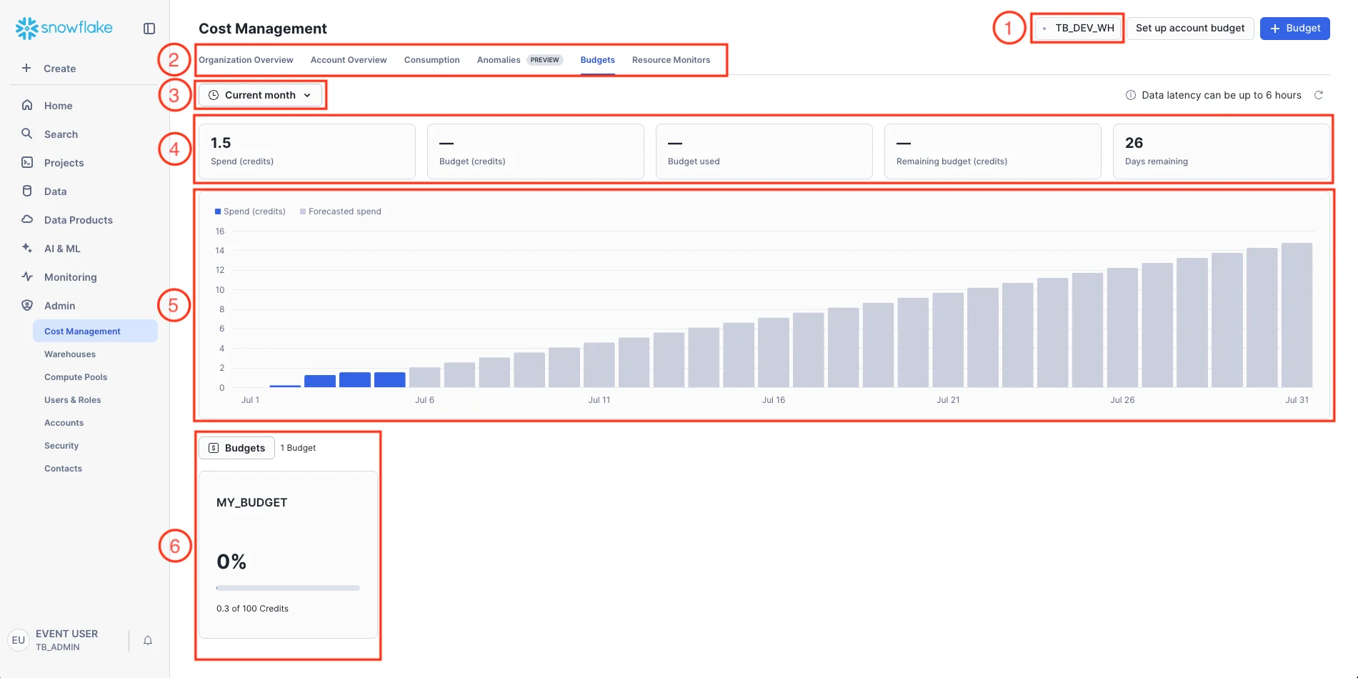
Let's take a look at the Budget Page on Snowsight.
Navigate to
Admin
»
Cost Management
»
Budgets
.
9/26/26, 12:02 PM
Zero to Snowflake
https://www.snowflake.com/en/developers/guides/zero-to-snowflake/
8/59
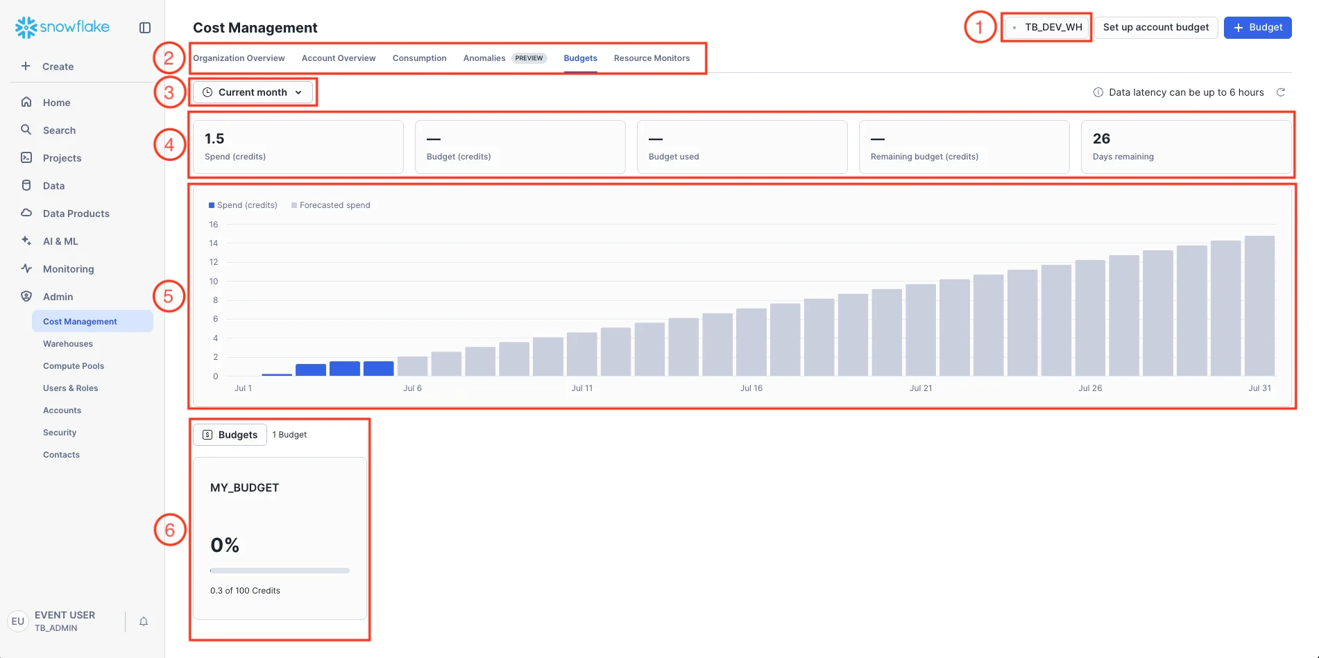
Step 3 - Configuring the Budget in Snowsight
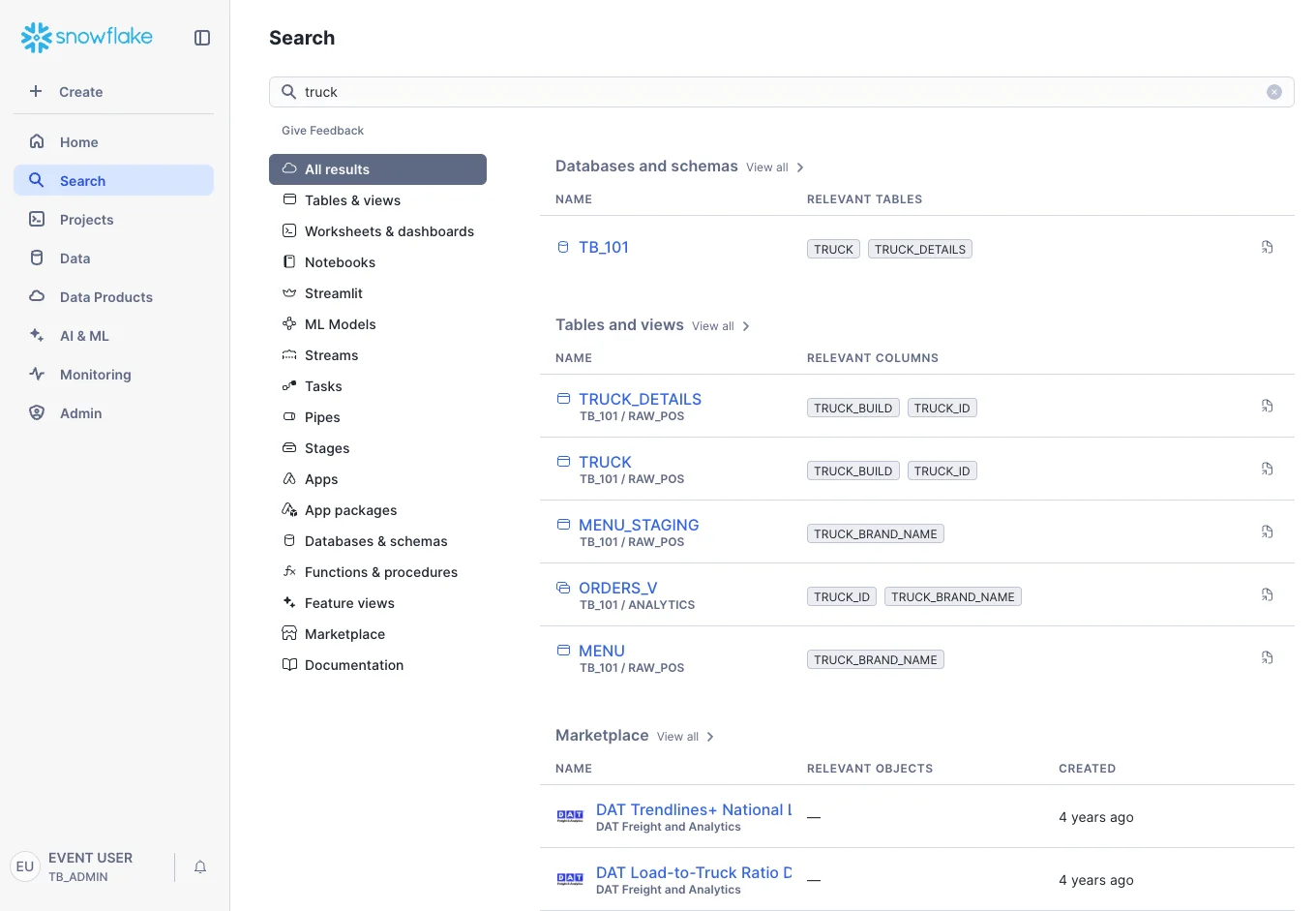
Key:
1. Warehouse Context
2. Cost Management Navigation
3. Time Period Filter
4. Key Metrics Summary
5. Spend and Forecast Trend Chart
6. Budget Details
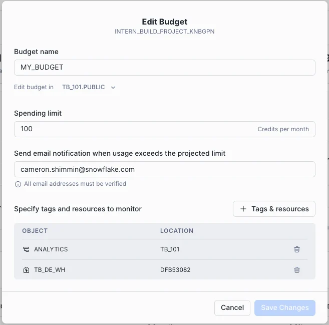
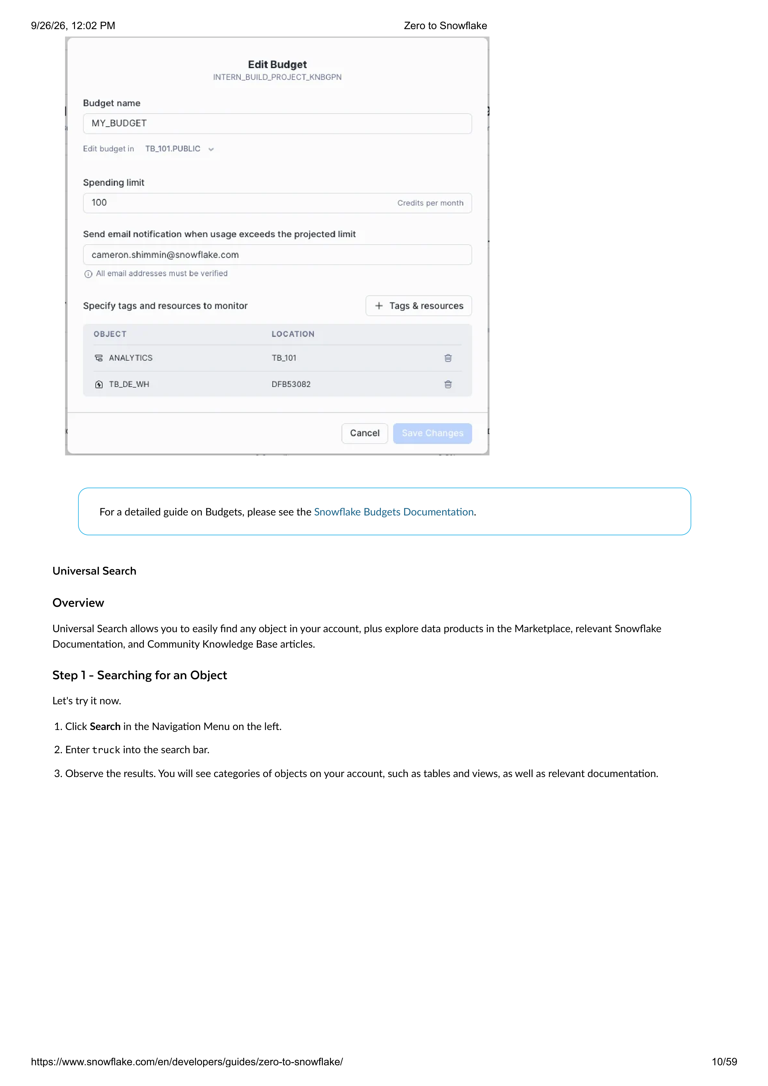
Configuring a budget is done through the Snowsight UI.
1. Make sure your account role is set to
ACCOUNTADMIN
. You can change this in the bottom left corner.
2. Click on the
MY_BUDGET
budget we created.
3. Click
Budget Details
to open the Budget details panel, then click
Edit
in the Budget Details panel on the right.
4. Set the
Spending Limit
to
100
.
5. Enter a verified notification email address.
6. Click
+ Tags & Resources
and add the
TB_101.ANALYTICS
schema and the
TB_DE_WH
warehouse to be monitored.
7. Click
Save Changes
.
9/26/26, 12:02 PM
Zero to Snowflake
https://www.snowflake.com/en/developers/guides/zero-to-snowflake/
9/59
Universal Search
Overview
Step 1 - Searching for an Object
For a detailed guide on Budgets, please see the
Snowflake Budgets Documentation
.
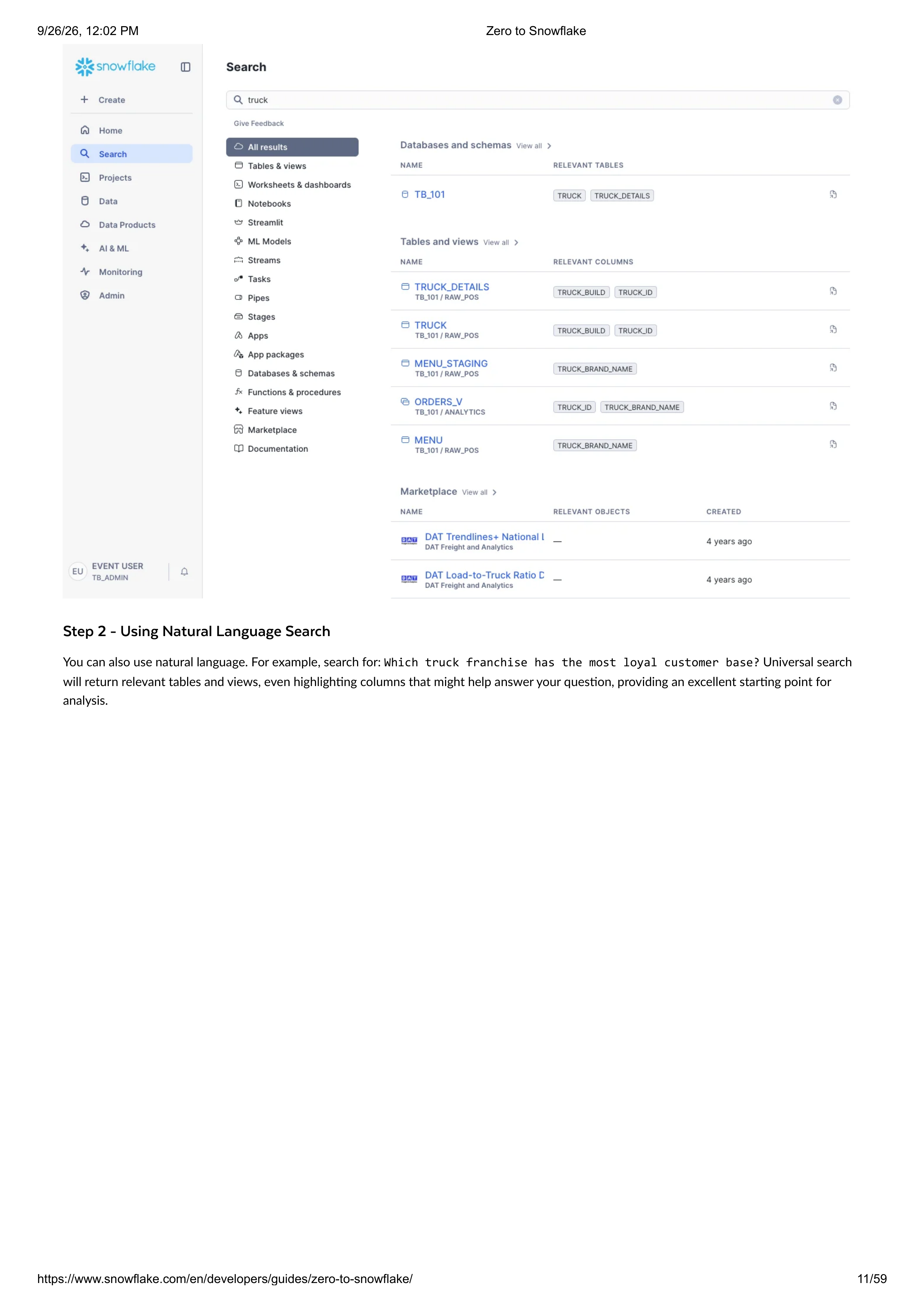
Universal Search allows you to easily find any object in your account, plus explore data products in the Marketplace, relevant Snowflake
Documentation, and Community Knowledge Base articles.
Let's try it now.
1. Click
Search
in the Navigation Menu on the left.
2. Enter
truck
into the search bar.
3. Observe the results. You will see categories of objects on your account, such as tables and views, as well as relevant documentation.
9/26/26, 12:02 PM
Zero to Snowflake
https://www.snowflake.com/en/developers/guides/zero-to-snowflake/
10/59
Step 2 - Using Natural Language Search
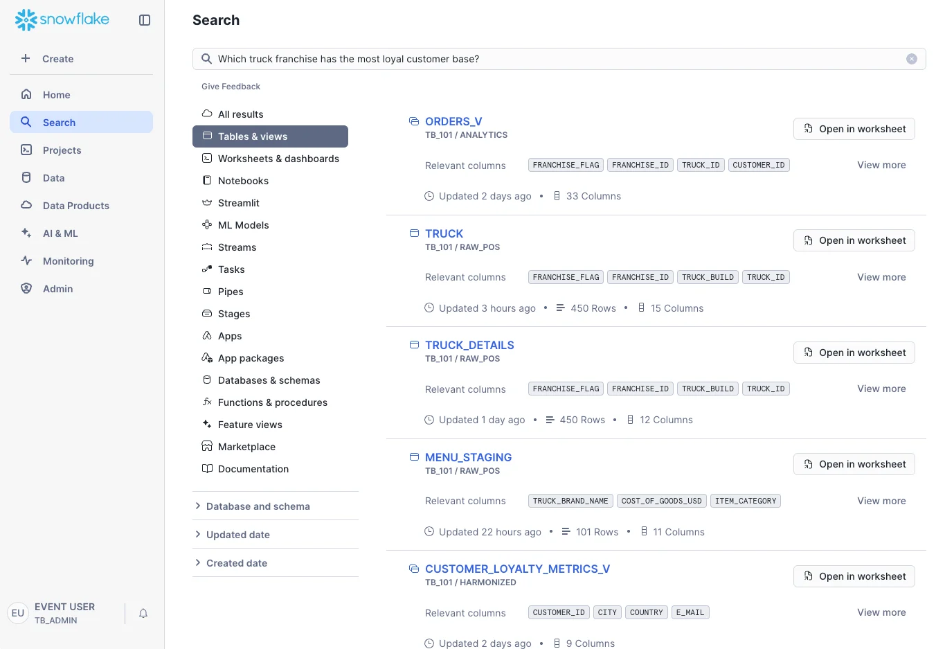
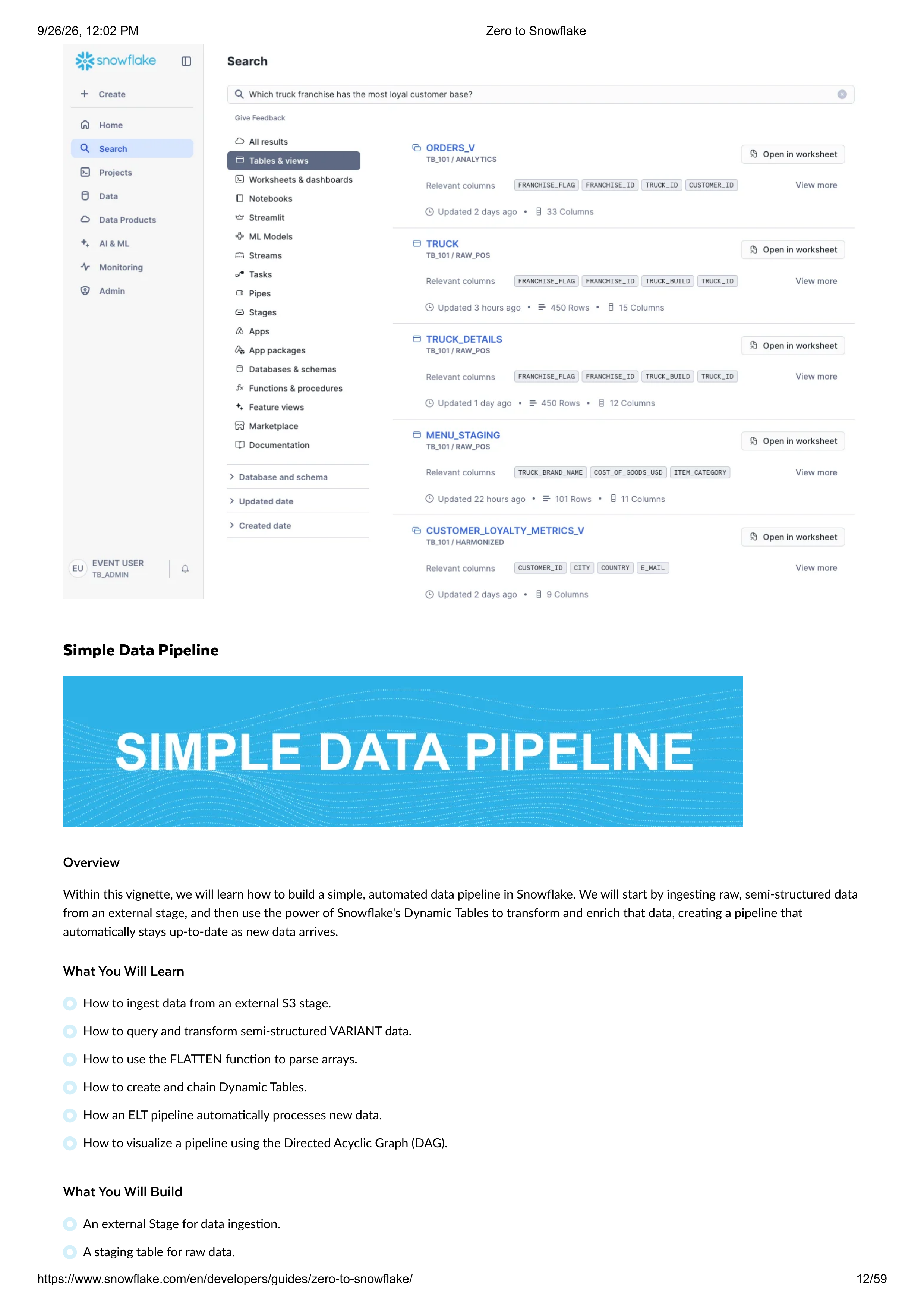
You can also use natural language. For example, search for:
Which truck franchise has the most loyal customer base?
Universal search
will return relevant tables and views, even highlighting columns that might help answer your question, providing an excellent starting point for
analysis.
9/26/26, 12:02 PM
Zero to Snowflake
https://www.snowflake.com/en/developers/guides/zero-to-snowflake/
11/59

Simple Data Pipeline
Overview
What You Will Learn
What You Will Build
Within this vignette, we will learn how to build a simple, automated data pipeline in Snowflake. We will start by ingesting raw, semi-structured data
from an external stage, and then use the power of Snowflake's Dynamic Tables to transform and enrich that data, creating a pipeline that
automatically stays up-to-date as new data arrives.
How to ingest data from an external S3 stage.
How to query and transform semi-structured VARIANT data.
How to use the FLATTEN function to parse arrays.
How to create and chain Dynamic Tables.
How an ELT pipeline automatically processes new data.
How to visualize a pipeline using the Directed Acyclic Graph (DAG).
An external Stage for data ingestion.
A staging table for raw data.
9/26/26, 12:02 PM
Zero to Snowflake
https://www.snowflake.com/en/developers/guides/zero-to-snowflake/
12/59
Get the SQL and paste it into your SQL File.
External Stage Ingestion
Overview
Step 1 - Set Context
Step 2 - Create Stage and Staging Table
Step 3 - Copy Data into Staging Table
A multi-step data pipeline using three chained Dynamic Tables.
Copy and paste the SQL from this
file
in a new SQL File to follow along in Snowflake. Note that once you've reached the end of the SQL File you
can skip to Step 16 - Snowflake Cortex AI.
Our raw menu data currently sits in an Amazon S3 bucket as CSV files. To begin our pipeline, we first need to ingest this data into Snowflake. We
will do this by creating a Stage to point to the S3 bucket and then using the
COPY
command to load the data into a staging table.
First, let's set our session context to use the correct database, role, and warehouse. Execute the first few queries in your SQL file.
ALTER SESSION SET query_tag = '{"origin":"sf_sit-is","name":"tb_zts","version":{"major":1, "minor":1},"attribu
ALTER SESSION SET query_tag = '{"origin":"sf_sit-is","name":"tb_zts","version":{"major":1, "minor":1},"attribu
USE DATABASE tb_101;
USE DATABASE tb_101;
USE ROLE tb_data_engineer;
USE ROLE tb_data_engineer;
USE WAREHOUSE tb_de_wh;
USE WAREHOUSE tb_de_wh;
A Stage is a Snowflake object that specifies an external location where data files are stored. We'll create a stage that points to our public S3 bucket.
Then, we'll create the table that will hold this raw data.
-- Create the menu stage
-- Create the menu stage
CREATE OR REPLACE STAGE raw_pos.menu_stage
CREATE OR REPLACE STAGE raw_pos.menu_stage
COMMENT = 'Stage for menu data'
COMMENT = 'Stage for menu data'
URL = 's3://sfquickstarts/frostbyte_tastybytes/raw_pos/menu/'
URL = 's3://sfquickstarts/frostbyte_tastybytes/raw_pos/menu/'
FILE_FORMAT = public.csv_ff;
FILE_FORMAT = public.csv_ff;
CREATE OR REPLACE TABLE raw_pos.menu_staging
CREATE OR REPLACE TABLE raw_pos.menu_staging
(
menu_id NUMBER(19,0),
menu_id NUMBER(19,0),
menu_type_id NUMBER(38,0),
menu_type_id NUMBER(38,0),
menu_type VARCHAR(16777216),
menu_type VARCHAR(16777216),
truck_brand_name VARCHAR(16777216),
truck_brand_name VARCHAR(16777216),
menu_item_id NUMBER(38,0),
menu_item_id NUMBER(38,0),
menu_item_name VARCHAR(16777216),
menu_item_name VARCHAR(16777216),
item_category VARCHAR(16777216),
item_category VARCHAR(16777216),
item_subcategory VARCHAR(16777216),
item_subcategory VARCHAR(16777216),
cost_of_goods_usd NUMBER(38,4),
cost_of_goods_usd NUMBER(38,4),
sale_price_usd NUMBER(38,4),
sale_price_usd NUMBER(38,4),
menu_item_health_metrics_obj VARIANT
menu_item_health_metrics_obj VARIANT
);
);
With the stage and table in place, let's load the data from the stage into our
menu_staging
table using the
COPY INTO
command.
COPY INTO raw_pos.menu_staging
COPY INTO raw_pos.menu_staging
FROM @raw_pos.menu_stage;
FROM @raw_pos.menu_stage;
COPY INTO TABLE
: This powerful command loads data from a staged file into a Snowflake table. It is the primary method for
bulk data ingestion.
9/26/26, 12:02 PM
Zero to Snowflake
https://www.snowflake.com/en/developers/guides/zero-to-snowflake/
13/59
Semi-Structured Data
Overview
Step 1 - Querying VARIANT Data
Step 2 - Parsing Arrays with FLATTEN
Dynamic Tables
Overview
Step 1 - Creating the First Dynamic Table
Snowflake excels at handling semi-structured data like JSON using its native
VARIANT
data type. One of the columns we ingested,
menu_item_health_metrics_obj
, contains JSON. Let's explore how to query it.
Let's look at the raw JSON. Notice it contains nested objects and arrays.
SELECT menu_item_health_metrics_obj FROM raw_pos.menu_staging;
SELECT menu_item_health_metrics_obj FROM raw_pos.menu_staging;
We can use special syntax to navigate the JSON structure. The colon (
:
) accesses keys by name, and square brackets (
[]
) access array elements by
index. We can also cast results to explicit data types using the
CAST
function or the double-colon shorthand (
::
).
SELECT
SELECT
menu_item_name,
menu_item_name,
CAST(menu_item_health_metrics_obj:menu_item_id AS INTEGER) AS menu_item_id, -- Casting using 'AS'
CAST(menu_item_health_metrics_obj:menu_item_id AS INTEGER) AS menu_item_id, -- Casting using 'AS'
menu_item_health_metrics_obj:menu_item_health_metrics[0]:ingredients::ARRAY AS ingredients -- Casting usin
menu_item_health_metrics_obj:menu_item_health_metrics[0]:ingredients::ARRAY AS ingredients -- Casting usin
FROM raw_pos.menu_staging;
FROM raw_pos.menu_staging;
The
FLATTEN
function is a powerful tool for un-nesting arrays. It produces a new row for each element in an array. Let's use it to create a list of
every ingredient for every menu item.
SELECT
SELECT
i.value::STRING AS ingredient_name,
i.value::STRING AS ingredient_name,
m.menu_item_health_metrics_obj:menu_item_id::INTEGER AS menu_item_id
m.menu_item_health_metrics_obj:menu_item_id::INTEGER AS menu_item_id
FROM
FROM
raw_pos.menu_staging m,
raw_pos.menu_staging m,
LATERAL FLATTEN(INPUT => m.menu_item_health_metrics_obj:menu_item_health_metrics[0]:ingredients::ARRAY) i;
LATERAL FLATTEN(INPUT => m.menu_item_health_metrics_obj:menu_item_health_metrics[0]:ingredients::ARRAY) i;
Semi-Structured Data Types
: Snowflake's VARIANT, OBJECT, and ARRAY types allow you to store and query semi-structured
data directly, without needing to define a rigid schema upfront.
Our franchises are constantly adding new menu items. We need a way to process this new data automatically. For this, we can use Dynamic Tables,
a powerful tool designed to simplify data transformation pipelines by declaratively defining the result of a query and letting Snowflake handle the
refreshes.
We'll start by creating a dynamic table that extracts all unique ingredients from our staging table. We set a
LAG
of '1 minute', which tells Snowflake
the maximum amount of time this table's data can be behind the source data.
CREATE OR REPLACE DYNAMIC TABLE harmonized.ingredient
CREATE OR REPLACE DYNAMIC TABLE harmonized.ingredient
LAG = '1 minute'
LAG = '1 minute'
WAREHOUSE = 'TB_DE_WH'
WAREHOUSE = 'TB_DE_WH'
AS
AS
SELECT
SELECT
ingredient_name,
ingredient_name,
menu_ids
menu_ids
FROM (
FROM (
SELECT DISTINCT
SELECT DISTINCT
i.value::STRING AS ingredient_name,
i.value::STRING AS ingredient_name,
9/26/26, 12:02 PM
Zero to Snowflake
https://www.snowflake.com/en/developers/guides/zero-to-snowflake/
14/59
Step 2 - Testing the Automatic Refresh
Build Out the Pipeline
Overview
Step 1 - Creating a Lookup Table
Step 2 - Adding Transactional Data
ARRAY_AGG(m.menu_item_id) AS menu_ids
ARRAY_AGG(m.menu_item_id) AS menu_ids
FROM
FROM
raw_pos.menu_staging m,
raw_pos.menu_staging m,
LATERAL FLATTEN(INPUT => menu_item_health_metrics_obj:menu_item_health_metrics[0]:ingredients::ARRAY)
LATERAL FLATTEN(INPUT => menu_item_health_metrics_obj:menu_item_health_metrics[0]:ingredients::ARRAY)
GROUP BY i.value::STRING
GROUP BY i.value::STRING
);
);
Dynamic Tables
: Dynamic Tables automatically refresh as their underlying source data changes, simplifying ELT pipelines and
ensuring data freshness without manual intervention or complex scheduling.
Let's see the automation in action. One of our trucks has added a Banh Mi sandwich, which contains new ingredients for French Baguette and
Pickled Daikon. Let's insert this new menu item into our staging table.
INSERT INTO raw_pos.menu_staging
INSERT INTO raw_pos.menu_staging
SELECT
SELECT
10101, 15, 'Sandwiches', 'Better Off Bread', 157, 'Banh Mi', 'Main', 'Cold Option', 9.0, 12.0,
10101, 15, 'Sandwiches', 'Better Off Bread', 157, 'Banh Mi', 'Main', 'Cold Option', 9.0, 12.0,
PARSE_JSON('{"menu_item_health_metrics": [{"ingredients": ["French Baguette","Mayonnaise","Pickled Daikon"
PARSE_JSON('{"menu_item_health_metrics": [{"ingredients": ["French Baguette","Mayonnaise","Pickled Daikon"
Now, query the
harmonized.ingredient
table. Within a minute, you should see the new ingredients appear automatically.
-- You may need to wait up to 1 minute and re-run this query
-- You may need to wait up to 1 minute and re-run this query
SELECT * FROM harmonized.ingredient
SELECT * FROM harmonized.ingredient
WHERE ingredient_name IN ('French Baguette', 'Pickled Daikon');
WHERE ingredient_name IN ('French Baguette', 'Pickled Daikon');
Now we can build a multi-step pipeline by creating more dynamic tables that read from other dynamic tables. This creates a chain, or a Directed
Acyclic Graph (DAG), where updates automatically flow from the source to the final output.
Let's create a lookup table that maps ingredients to the menu items they are used in. This dynamic table reads from our
harmonized.ingredient
dynamic table.
CREATE OR REPLACE DYNAMIC TABLE harmonized.ingredient_to_menu_lookup
CREATE OR REPLACE DYNAMIC TABLE harmonized.ingredient_to_menu_lookup
LAG = '1 minute'
LAG = '1 minute'
WAREHOUSE = 'TB_DE_WH'
WAREHOUSE = 'TB_DE_WH'
AS
AS
SELECT
SELECT
i.ingredient_name,
i.ingredient_name,
m.menu_item_health_metrics_obj:menu_item_id::INTEGER AS menu_item_id
m.menu_item_health_metrics_obj:menu_item_id::INTEGER AS menu_item_id
FROM
FROM
raw_pos.menu_staging m,
raw_pos.menu_staging m,
LATERAL FLATTEN(INPUT => m.menu_item_health_metrics_obj:menu_item_health_metrics[0]:ingredients) f
LATERAL FLATTEN(INPUT => m.menu_item_health_metrics_obj:menu_item_health_metrics[0]:ingredients) f
JOIN harmonized.ingredient i ON f.value::STRING = i.ingredient_name;
JOIN harmonized.ingredient i ON f.value::STRING = i.ingredient_name;
Let's simulate an order of two Banh Mi sandwiches by inserting records into our order tables.
INSERT INTO raw_pos.order_header
INSERT INTO raw_pos.order_header
SELECT
SELECT
459520441, 15, 1030, 101565, null, 200322900,
459520441, 15, 1030, 101565, null, 200322900,
TO_TIMESTAMP_NTZ('08:00:00', 'hh:mi:ss'),
TO_TIMESTAMP_NTZ('08:00:00', 'hh:mi:ss'),
TO_TIMESTAMP_NTZ('14:00:00', 'hh:mi:ss'),
TO_TIMESTAMP_NTZ('14:00:00', 'hh:mi:ss'),
9/26/26, 12:02 PM
Zero to Snowflake
https://www.snowflake.com/en/developers/guides/zero-to-snowflake/
15/59
Step 3 - Creating the Final Pipeline Table
Step 4 - Querying the Final Output
Visualize the Pipeline
Overview
null, TO_TIMESTAMP_NTZ('2022-01-27 08:21:08.000'),
null, TO_TIMESTAMP_NTZ('2022-01-27 08:21:08.000'),
null, 'USD', 14.00, null, null, 14.00;
null, 'USD', 14.00, null, null, 14.00;
INSERT INTO raw_pos.order_detail
INSERT INTO raw_pos.order_detail
SELECT
SELECT
904745311, 459520441, 157, null, 0, 2, 14.00, 28.00, null;
904745311, 459520441, 157, null, 0, 2, 14.00, 28.00, null;
Finally, let's create our final dynamic table. This one joins our order data with our ingredient lookup tables to create a summary of monthly
ingredient usage per truck. This table depends on the other dynamic tables, completing our pipeline.
CREATE OR REPLACE DYNAMIC TABLE harmonized.ingredient_usage_by_truck
CREATE OR REPLACE DYNAMIC TABLE harmonized.ingredient_usage_by_truck
LAG = '2 minute'
LAG = '2 minute'
WAREHOUSE = 'TB_DE_WH'
WAREHOUSE = 'TB_DE_WH'
AS
AS
SELECT
SELECT
oh.truck_id,
oh.truck_id,
EXTRACT(YEAR FROM oh.order_ts) AS order_year,
EXTRACT(YEAR FROM oh.order_ts) AS order_year,
MONTH(oh.order_ts) AS order_month,
MONTH(oh.order_ts) AS order_month,
i.ingredient_name,
i.ingredient_name,
SUM(od.quantity) AS total_ingredients_used
SUM(od.quantity) AS total_ingredients_used
FROM
FROM
raw_pos.order_detail od
raw_pos.order_detail od
JOIN raw_pos.order_header oh ON od.order_id = oh.order_id
JOIN raw_pos.order_header oh ON od.order_id = oh.order_id
JOIN harmonized.ingredient_to_menu_lookup iml ON od.menu_item_id = iml.menu_item_id
JOIN harmonized.ingredient_to_menu_lookup iml ON od.menu_item_id = iml.menu_item_id
JOIN harmonized.ingredient i ON iml.ingredient_name = i.ingredient_name
JOIN harmonized.ingredient i ON iml.ingredient_name = i.ingredient_name
JOIN raw_pos.location l ON l.location_id = oh.location_id
JOIN raw_pos.location l ON l.location_id = oh.location_id
WHERE l.country = 'United States'
WHERE l.country = 'United States'
GROUP BY
GROUP BY
oh.truck_id,
oh.truck_id,
order_year,
order_year,
order_month,
order_month,
i.ingredient_name
i.ingredient_name
ORDER BY
ORDER BY
oh.truck_id,
oh.truck_id,
total_ingredients_used DESC;
total_ingredients_used DESC;
Now, let's query the final table in our pipeline. After a few minutes for the refreshes to complete, you will see the ingredient usage for two Banh
Mis from the order we inserted in a previous step. The entire pipeline updated automatically.
-- You may need to wait up to 2 minutes and re-run this query
-- You may need to wait up to 2 minutes and re-run this query
SELECT
SELECT
truck_id,
truck_id,
ingredient_name,
ingredient_name,
SUM(total_ingredients_used) AS total_ingredients_used
SUM(total_ingredients_used) AS total_ingredients_used
FROM
FROM
harmonized.ingredient_usage_by_truck
harmonized.ingredient_usage_by_truck
WHERE
WHERE
order_month = 1
order_month = 1
AND truck_id = 15
AND truck_id = 15
GROUP BY truck_id, ingredient_name
GROUP BY truck_id, ingredient_name
ORDER BY total_ingredients_used DESC;
ORDER BY total_ingredients_used DESC;
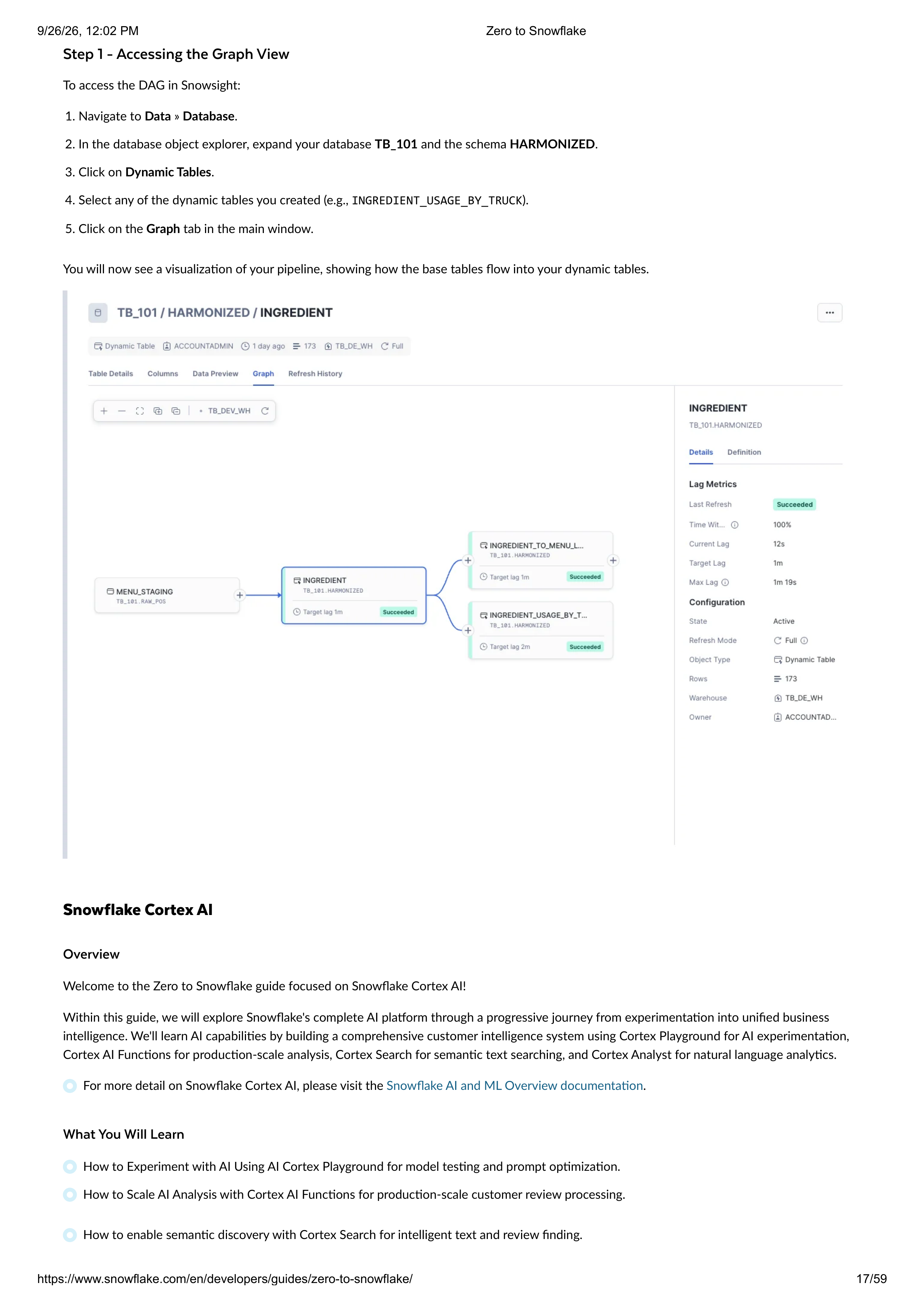
Finally, let's visualize our pipeline's Directed Acyclic Graph, or DAG. The DAG shows how our data flows through the tables, and it can be used to
monitor the health and lag of our pipeline.
9/26/26, 12:02 PM
Zero to Snowflake
https://www.snowflake.com/en/developers/guides/zero-to-snowflake/
16/59
Step 1 - Accessing the Graph View
Snowflake Cortex AI
Overview
What You Will Learn
To access the DAG in Snowsight:
1. Navigate to
Data
»
Database
.
2. In the database object explorer, expand your database
TB_101
and the schema
HARMONIZED
.
3. Click on
Dynamic Tables
.
4. Select any of the dynamic tables you created (e.g.,
INGREDIENT_USAGE_BY_TRUCK
).
5. Click on the
Graph
tab in the main window.
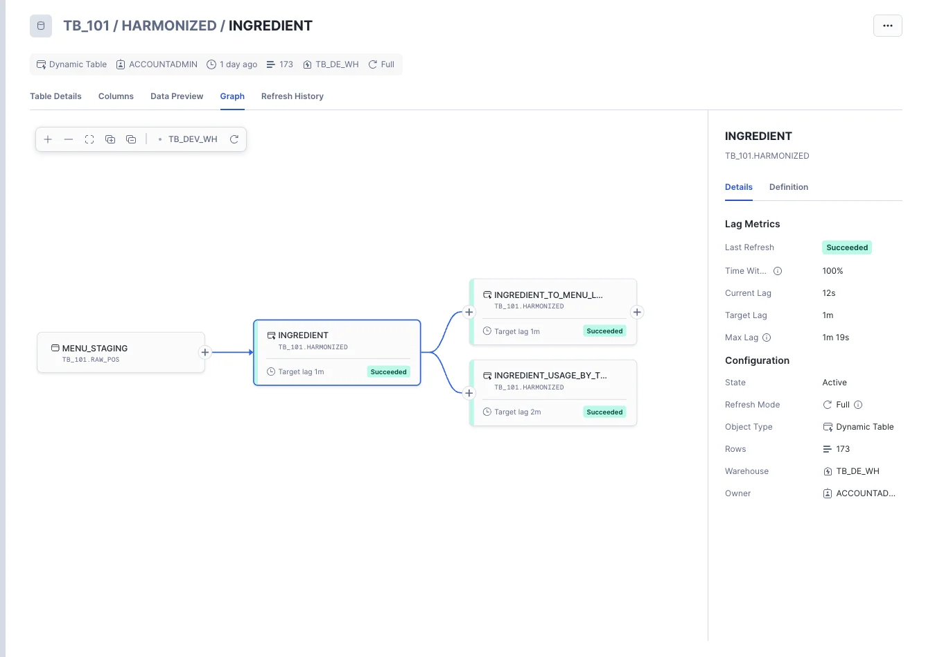
You will now see a visualization of your pipeline, showing how the base tables flow into your dynamic tables.
Welcome to the Zero to Snowflake guide focused on Snowflake Cortex AI!
Within this guide, we will explore Snowflake's complete AI platform through a progressive journey from experimentation into unified business
intelligence. We'll learn AI capabilities by building a comprehensive customer intelligence system using Cortex Playground for AI experimentation,
Cortex AI Functions for production-scale analysis, Cortex Search for semantic text searching, and Cortex Analyst for natural language analytics.
For more detail on Snowflake Cortex AI, please visit the
Snowflake AI and ML Overview documentation
.
How to Experiment with AI Using AI Cortex Playground for model testing and prompt optimization.
How to Scale AI Analysis with Cortex AI Functions for production-scale customer review processing.
How to enable semantic discovery with Cortex Search for intelligent text and review finding.
9/26/26, 12:02 PM
Zero to Snowflake
https://www.snowflake.com/en/developers/guides/zero-to-snowflake/
17/59

What You Will Build
Cortex Playground
Overview
Step 1 - Connect Data & Filter
How to create conversational analytics with Cortex Analyst for natural language business intelligence.
Through this journey, you’ll construct a complete intelligence customer analytics platform:
Phase 1: AI Foundation
AI Experimentation Environment using Cortex Playground for model testing and optimization.
Production-scale Review Analysis pipeline using Cortex AI Functions for systematic customer feedback processing.
Phase 2: Intelligent Development & Discovery
Semantic Search Engine using Cortex Search for instant customer feedback discovery and operational intelligence.
Phase 3: Conversational Intelligence
Natural Language Business Analytics Interface using Cortex Analyst for conversational data exploration.
Unified AI Business Intelligence Platform using Snowflake CoWork that connects customer voice with business performance
As a data analyst at Tasty Bytes, you need to rapidly explore customer feedback using AI models to identify service improvement opportunities.
Traditionally, AI experimentation is complex and time-consuming.
Snowflake Cortex Playground
solves this by offering a quick, secure environment
directly within Snowflake's UI to experiment with diverse AI models, compare their performance on real business data, and export successful
approaches as production-ready SQL. This module guides you through using Cortex Playground for rapid prototyping and seamless integration of AI
into your data workflows.
Let's begin by connecting directly to customer review data within Cortex Playground. This keeps your data secure within Snowflake while allowing
you to analyze feedback using AI models.
Navigation steps:
1. Navigate to
AI & ML → Studio → Cortex Playground
.
2. Select
Role: TB_DEV
and
Warehouse: TB_DEV_WH
.
3. Click "
+Connect your data
" in the prompt box.
4. Select data source:
5. Click
Let's go
6. Select text column:
REVIEW
.
7. Select filter column:
TRUCK_BRAND_NAME
.
8. Click
Done
.
9. In the system prompt box, apply a filter using the
TRUCK_BRAND_NAME
dropdown. There are multiple reviews available for each truck brand.
For instance, you can select "
Better Of Bread
" to narrow down the reviews. If "
Better Of Bread
" isn't available, please choose any other truck
brand from the dropdown and proceed with one of its reviews.
Database: TB_101
Schema: HARMONIZED
Table: TRUCK_REVIEWS_V
9/26/26, 12:02 PM
Zero to Snowflake
https://www.snowflake.com/en/developers/guides/zero-to-snowflake/
18/59

Step 2 - Compare AI Models for Insights
What you've accomplished:
You now have direct access to customer review data within the AI interface. The filter allows you
to focus your analysis on specific truck brands, making your experiment more targeted and relevant.
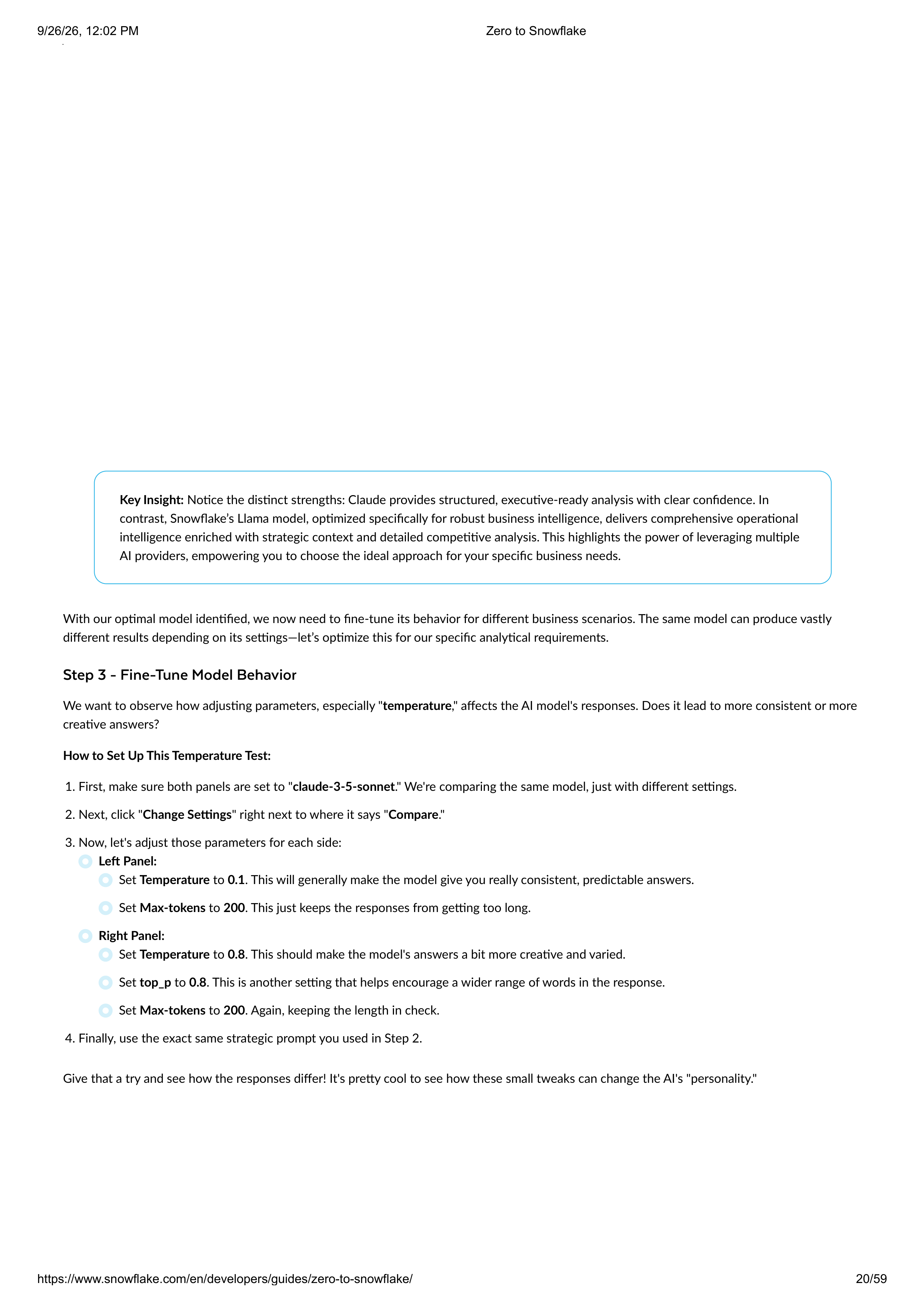
Now, let's analyze customer reviews to extract specific operational insights and compare how different AI models perform on this business task.
Setup Model Comparison:
1. Click "
Compare
" to enable side-by-side model comparison.
2. Set the left panel to "
claude-3-5-sonnet
" and the right panel to "
snowflake-llama-3.3-70b
".
Note:
Snowflake Cortex provides access to leading AI models from multiple providers, including Anthropic, OpenAI, Meta, and
others, giving you choice and flexibility without vendor lock-in.
Enter this strategic prompt:
Analyze this customer review across multiple dimensions: sentiment score with confidence level, key theme extraction,
competitive positioning insights, operational impact assessment, and priority ranking for management action
9/26/26, 12:02 PM
Zero to Snowflake
https://www.snowflake.com/en/developers/guides/zero-to-snowflake/
19/59

Step 3 - Fine-Tune Model Behavior
Key Insight:
Notice the distinct strengths: Claude provides structured, executive-ready analysis with clear confidence. In
contrast, Snowflake’s Llama model, optimized specifically for robust business intelligence, delivers comprehensive operational
intelligence enriched with strategic context and detailed competitive analysis. This highlights the power of leveraging multiple
AI providers, empowering you to choose the ideal approach for your specific business needs.
With our optimal model identified, we now need to fine-tune its behavior for different business scenarios. The same model can produce vastly
different results depending on its settings—let’s optimize this for our specific analytical requirements.
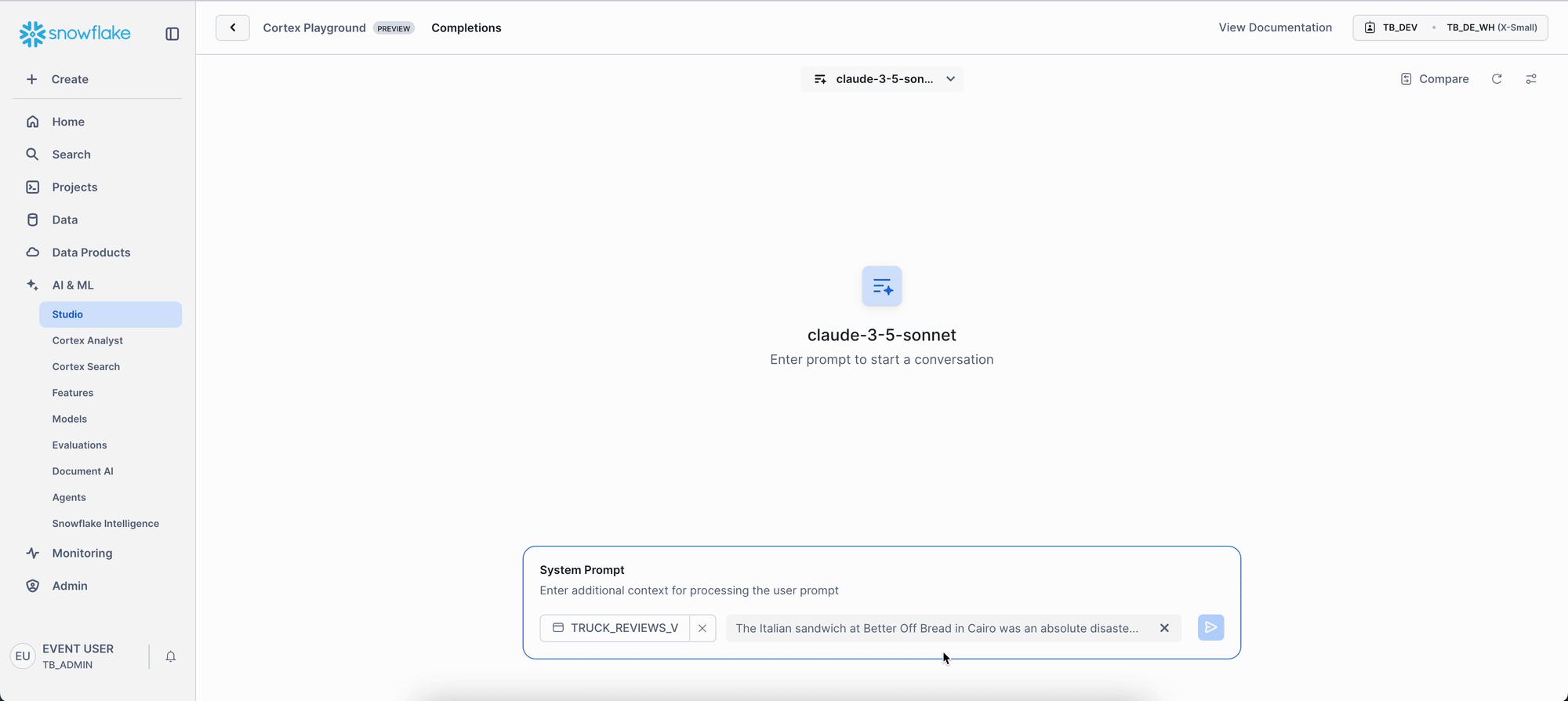
We want to observe how adjusting parameters, especially "
temperature
," affects the AI model's responses. Does it lead to more consistent or more
creative answers?
How to Set Up This Temperature Test:
1. First, make sure both panels are set to "
claude-3-5-sonnet
." We're comparing the same model, just with different settings.
2. Next, click "
Change Settings
" right next to where it says "
Compare
."
3. Now, let's adjust those parameters for each side:
4. Finally, use the exact same strategic prompt you used in Step 2.
Left Panel:
Set
Temperature
to
0.1
. This will generally make the model give you really consistent, predictable answers.
Set
Max-tokens
to
200
. This just keeps the responses from getting too long.
Right Panel:
Set
Temperature
to
0.8
. This should make the model's answers a bit more creative and varied.
Set
top_p
to
0.8
. This is another setting that helps encourage a wider range of words in the response.
Set
Max-tokens
to
200
. Again, keeping the length in check.
Give that a try and see how the responses differ! It's pretty cool to see how these small tweaks can change the AI's "personality."
9/26/26, 12:02 PM
Zero to Snowflake
https://www.snowflake.com/en/developers/guides/zero-to-snowflake/
20/59

Step 4 - Understanding the Underlying Technology
The Foundation: SQL at Its Core
Observe the Impact:
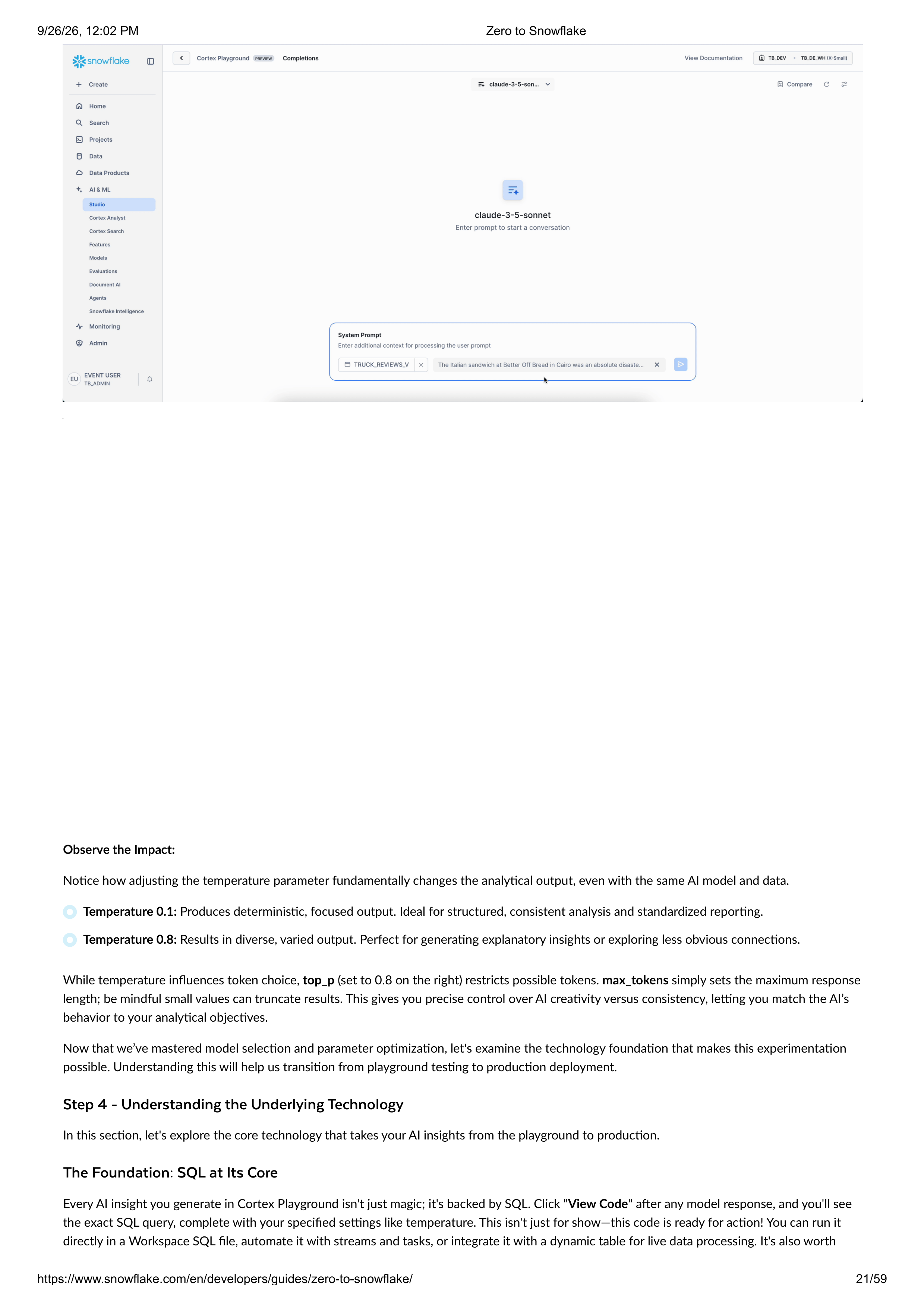
Notice how adjusting the temperature parameter fundamentally changes the analytical output, even with the same AI model and data.
Temperature 0.1:
Produces deterministic, focused output. Ideal for structured, consistent analysis and standardized reporting.
Temperature 0.8:
Results in diverse, varied output. Perfect for generating explanatory insights or exploring less obvious connections.
While temperature influences token choice,
top_p
(set to 0.8 on the right) restricts possible tokens.
max_tokens
simply sets the maximum response
length; be mindful small values can truncate results. This gives you precise control over AI creativity versus consistency, letting you match the AI’s
behavior to your analytical objectives.
Now that we’ve mastered model selection and parameter optimization, let's examine the technology foundation that makes this experimentation
possible. Understanding this will help us transition from playground testing to production deployment.
In this section, let's explore the core technology that takes your AI insights from the playground to production.
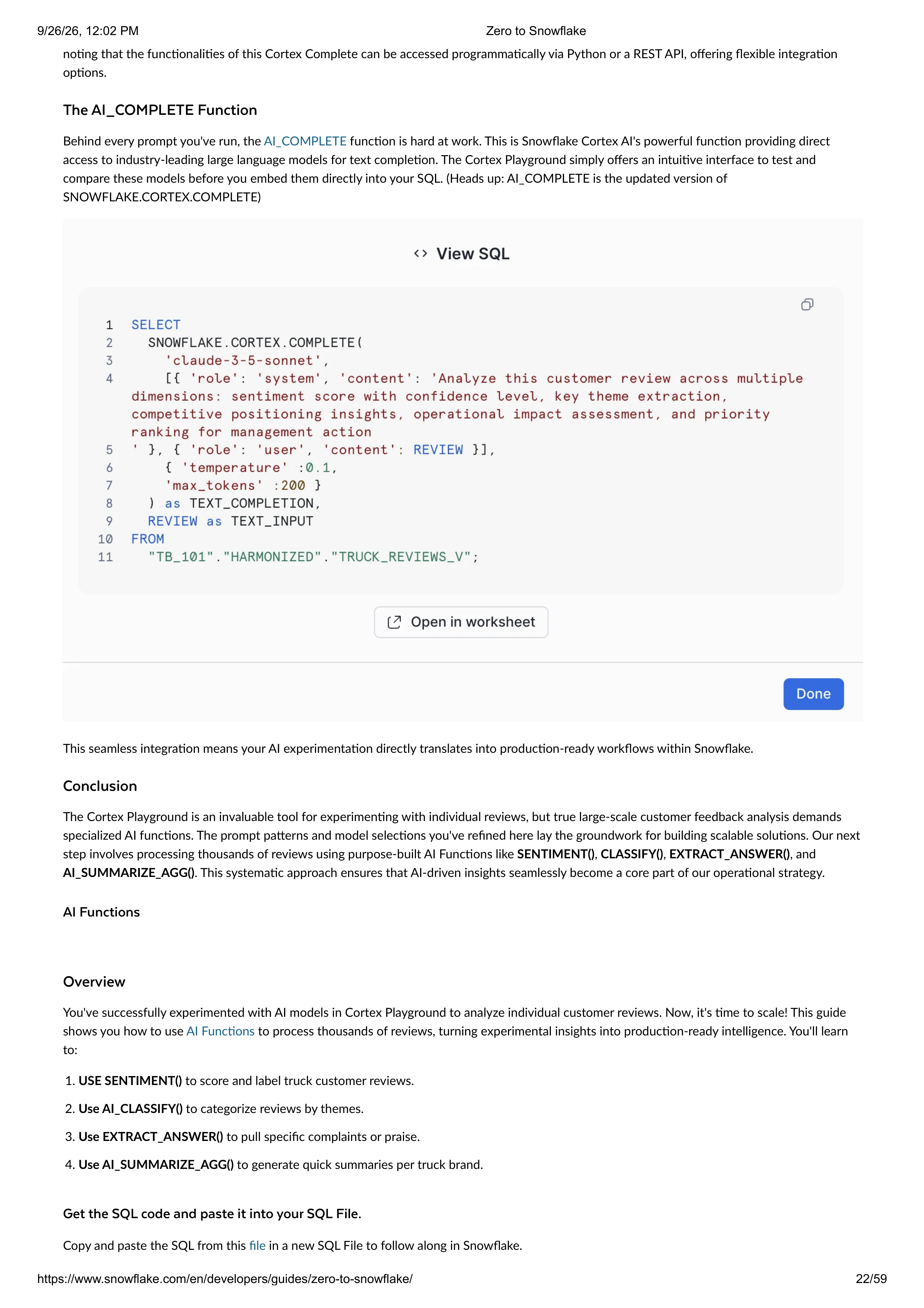
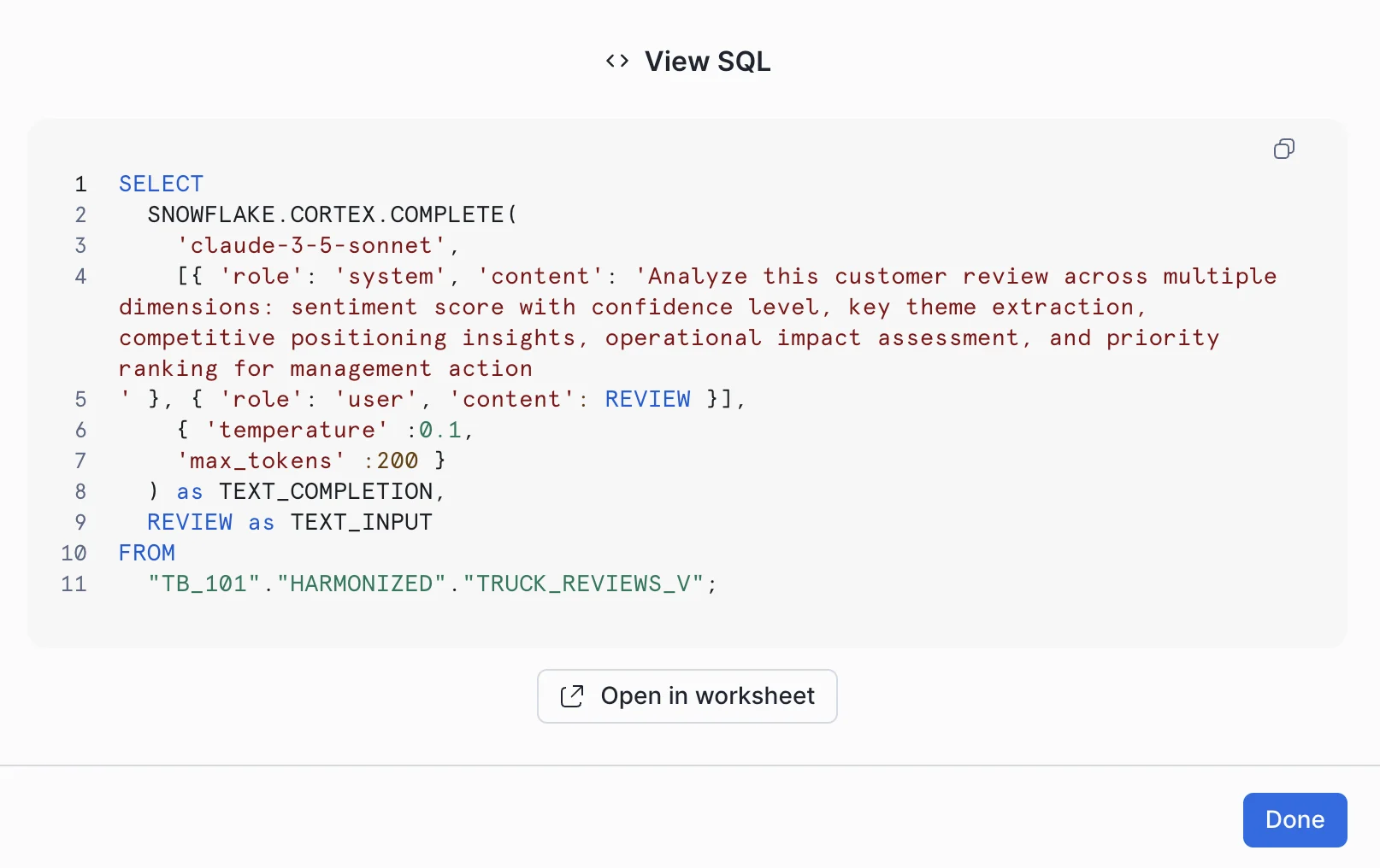
Every AI insight you generate in Cortex Playground isn't just magic; it's backed by SQL. Click "
View Code
" after any model response, and you'll see
the exact SQL query, complete with your specified settings like temperature. This isn't just for show—this code is ready for action! You can run it
directly in a Workspace SQL file, automate it with streams and tasks, or integrate it with a dynamic table for live data processing. It's also worth
9/26/26, 12:02 PM
Zero to Snowflake
https://www.snowflake.com/en/developers/guides/zero-to-snowflake/
21/59
The AI_COMPLETE Function
Conclusion
AI Functions
Overview
Get the SQL code and paste it into your SQL File.
noting that the functionalities of this Cortex Complete can be accessed programmatically via Python or a REST API, offering flexible integration
options.
Behind every prompt you've run, the
AI_COMPLETE
function is hard at work. This is Snowflake Cortex AI's powerful function providing direct
access to industry-leading large language models for text completion. The Cortex Playground simply offers an intuitive interface to test and
compare these models before you embed them directly into your SQL. (Heads up: AI_COMPLETE is the updated version of
SNOWFLAKE.CORTEX.COMPLETE)
This seamless integration means your AI experimentation directly translates into production-ready workflows within Snowflake.
The Cortex Playground is an invaluable tool for experimenting with individual reviews, but true large-scale customer feedback analysis demands
specialized AI functions. The prompt patterns and model selections you've refined here lay the groundwork for building scalable solutions. Our next
step involves processing thousands of reviews using purpose-built AI Functions like
SENTIMENT()
,
CLASSIFY()
,
EXTRACT_ANSWER()
, and
AI_SUMMARIZE_AGG()
. This systematic approach ensures that AI-driven insights seamlessly become a core part of our operational strategy.
You've successfully experimented with AI models in Cortex Playground to analyze individual customer reviews. Now, it's time to scale! This guide
shows you how to use
AI Functions
to process thousands of reviews, turning experimental insights into production-ready intelligence. You'll learn
to:
1.
USE SENTIMENT()
to score and label truck customer reviews.
2.
Use AI_CLASSIFY()
to categorize reviews by themes.
3.
Use EXTRACT_ANSWER()
to pull specific complaints or praise.
4.
Use AI_SUMMARIZE_AGG()
to generate quick summaries per truck brand.
Copy and paste the SQL from this
file
in a new SQL File to follow along in Snowflake.
9/26/26, 12:02 PM
Zero to Snowflake
https://www.snowflake.com/en/developers/guides/zero-to-snowflake/
22/59

Step 1 - Setting Context
Step 2 - Sentiment Analysis at Scale
First, let's set our session context. We will assume the role of a TastyBytes data analyst with the intention of leveraging AISQL functions to gain
insights from customer reviews.
ALTER SESSION SET query_tag = '{"origin":"sf_sit-is","name":"tb_zts","version":{"major":1, "minor":1},"attribu
ALTER SESSION SET query_tag = '{"origin":"sf_sit-is","name":"tb_zts","version":{"major":1, "minor":1},"attribu
USE ROLE tb_analyst;
USE ROLE tb_analyst;
USE DATABASE tb_101;
USE DATABASE tb_101;
USE WAREHOUSE tb_de_wh;
USE WAREHOUSE tb_de_wh;
Analyze customer sentiment across all food truck brands to identify which trucks are performing best and create fleet-wide customer satisfaction
metrics. In Cortex Playground, we analyzed individual reviews manually. Now we’ll use the
SENTIMENT()
function to automatically score customer
reviews from -1 (negative) to +1 (positive), following Snowflake's official sentiment ranges.
Business Question:
“How do customers feel about each of our truck brands overall?”
Please execute this query to analyze customer sentiment across our food truck network and categorize feedback.
SELECT
SELECT
truck_brand_name,
truck_brand_name,
COUNT(*) AS total_reviews,
COUNT(*) AS total_reviews,
AVG(CASE WHEN sentiment >= 0.5 THEN sentiment END) AS avg_positive_score,
AVG(CASE WHEN sentiment >= 0.5 THEN sentiment END) AS avg_positive_score,
AVG(CASE WHEN sentiment BETWEEN -0.5 AND 0.5 THEN sentiment END) AS avg_neutral_score,
AVG(CASE WHEN sentiment BETWEEN -0.5 AND 0.5 THEN sentiment END) AS avg_neutral_score,
AVG(CASE WHEN sentiment <= -0.5 THEN sentiment END) AS avg_negative_score
AVG(CASE WHEN sentiment <= -0.5 THEN sentiment END) AS avg_negative_score
FROM (
FROM (
SELECT
SELECT
truck_brand_name,
truck_brand_name,
SNOWFLAKE.CORTEX.SENTIMENT (review) AS sentiment
SNOWFLAKE.CORTEX.SENTIMENT (review) AS sentiment
FROM harmonized.truck_reviews_v
FROM harmonized.truck_reviews_v
WHERE
WHERE
language ILIKE '%en%'
language ILIKE '%en%'
AND review IS NOT NULL
AND review IS NOT NULL
LIMIT 10000
LIMIT 10000
)
GROUP BY
GROUP BY
truck_brand_name
truck_brand_name
ORDER BY total_reviews DESC;
ORDER BY total_reviews DESC;
9/26/26, 12:02 PM
Zero to Snowflake
https://www.snowflake.com/en/developers/guides/zero-to-snowflake/
23/59
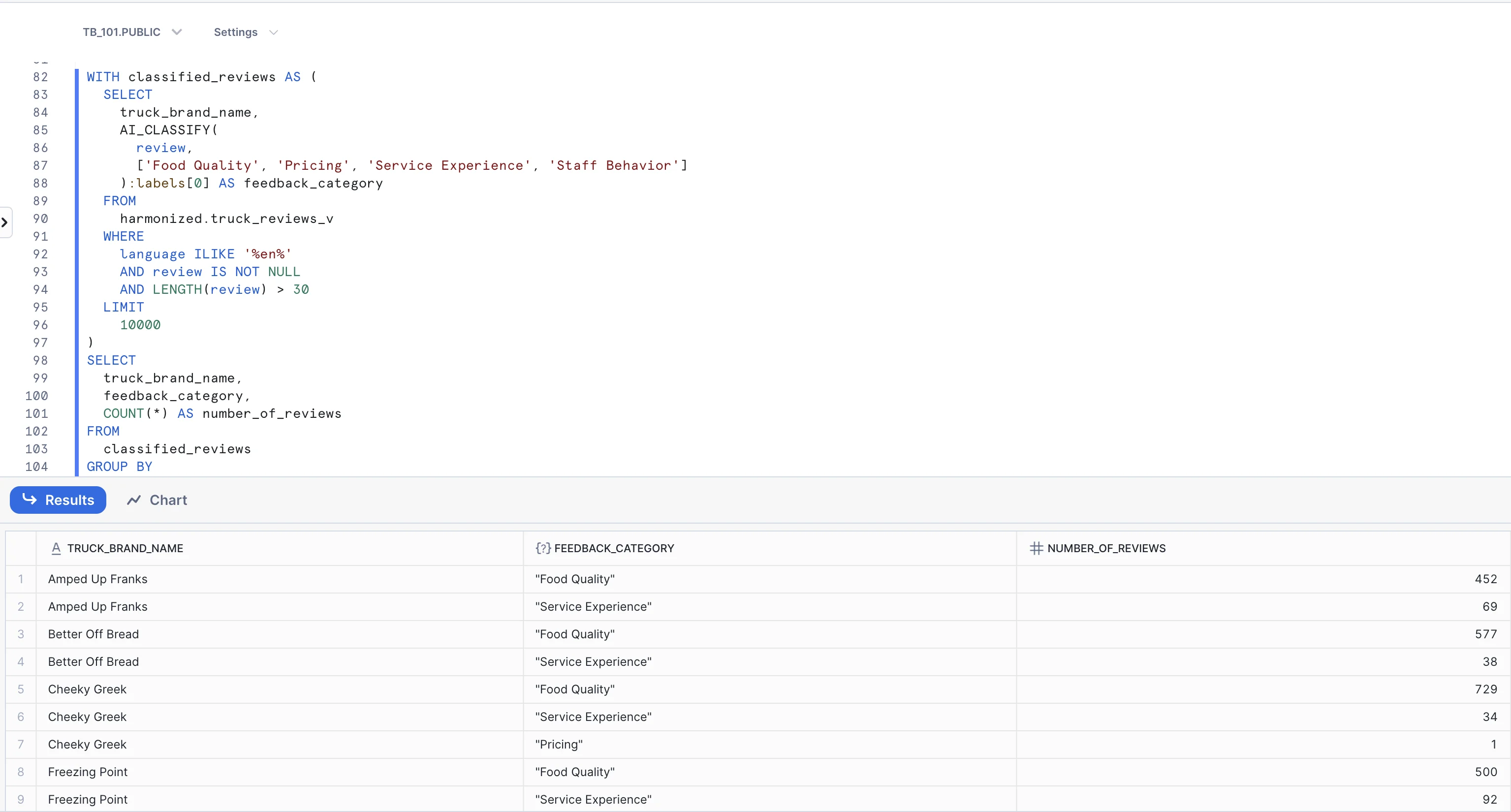
Step 3 - Categorize Customer Feedback
Key Insight
: Notice how we transitioned from analyzing reviews one at a time in Cortex Playground to systematically
processing thousands. The
SENTIMENT()
function automatically scored every review and categorized them into Positive,
Negative, and Neutral - giving us instant fleet-wide customer satisfaction metrics.
Sentiment Score Ranges
:
Positive: 0.5 to 1
Neutral: -0.5 to 0.5
Negative: -0.5 to -1
Now, let's categorize all reviews to understand what aspects of our service customers are talking about most. We'll use the
AI_CLASSIFY()
function, which automatically categorizes reviews into user-defined categories based on AI understanding, rather than simple keyword matching. In
this step, we will categorize customer feedback into business-relevant operational areas and analyze their distribution patterns.
Business Question:
“What are customers primarily commenting on - food quality, service, or delivery experience?"
Execute the Classification Query:
WITH classified_reviews AS (
WITH classified_reviews AS (
SELECT
SELECT
truck_brand_name,
truck_brand_name,
AI_CLASSIFY(
AI_CLASSIFY(
review,
review,
['Food Quality', 'Pricing', 'Service Experience', 'Staff Behavior']
['Food Quality', 'Pricing', 'Service Experience', 'Staff Behavior']
):labels[0] AS feedback_category
):labels[0] AS feedback_category
FROM
FROM
harmonized.truck_reviews_v
harmonized.truck_reviews_v
WHERE
WHERE
language ILIKE '%en%'
language ILIKE '%en%'
AND review IS NOT NULL
AND review IS NOT NULL
AND LENGTH(review) > 30
AND LENGTH(review) > 30
LIMIT
LIMIT
10000
10000
)
SELECT
SELECT
truck_brand_name,
truck_brand_name,
feedback_category,
feedback_category,
COUNT(*) AS number_of_reviews
COUNT(*) AS number_of_reviews
FROM
FROM
classified_reviews
classified_reviews
GROUP BY
GROUP BY
truck_brand_name,
truck_brand_name,
feedback_category
feedback_category
ORDER BY
ORDER BY
truck_brand_name,
truck_brand_name,
number_of_reviews DESC;
number_of_reviews DESC;
9/26/26, 12:02 PM
Zero to Snowflake
https://www.snowflake.com/en/developers/guides/zero-to-snowflake/
24/59
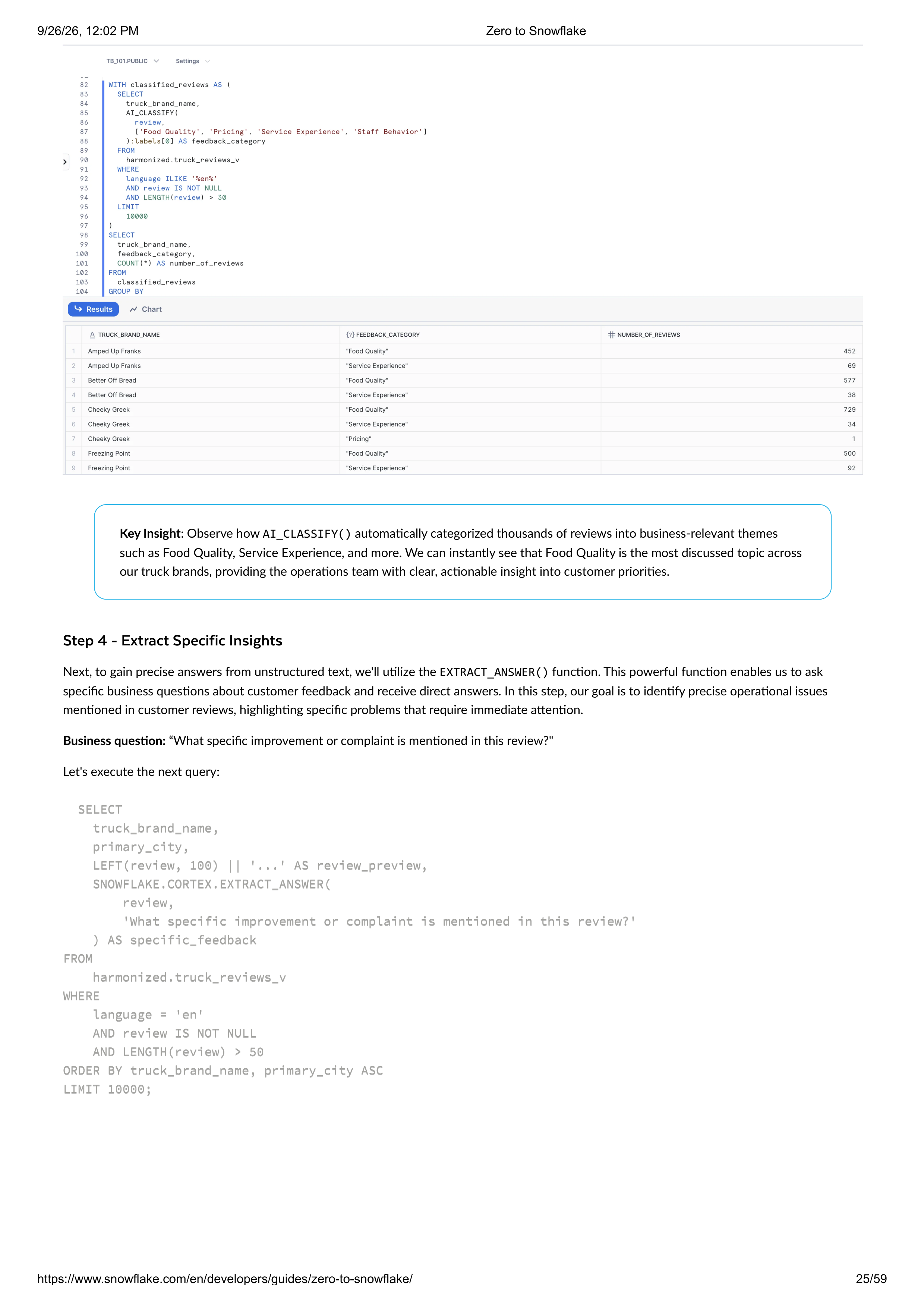
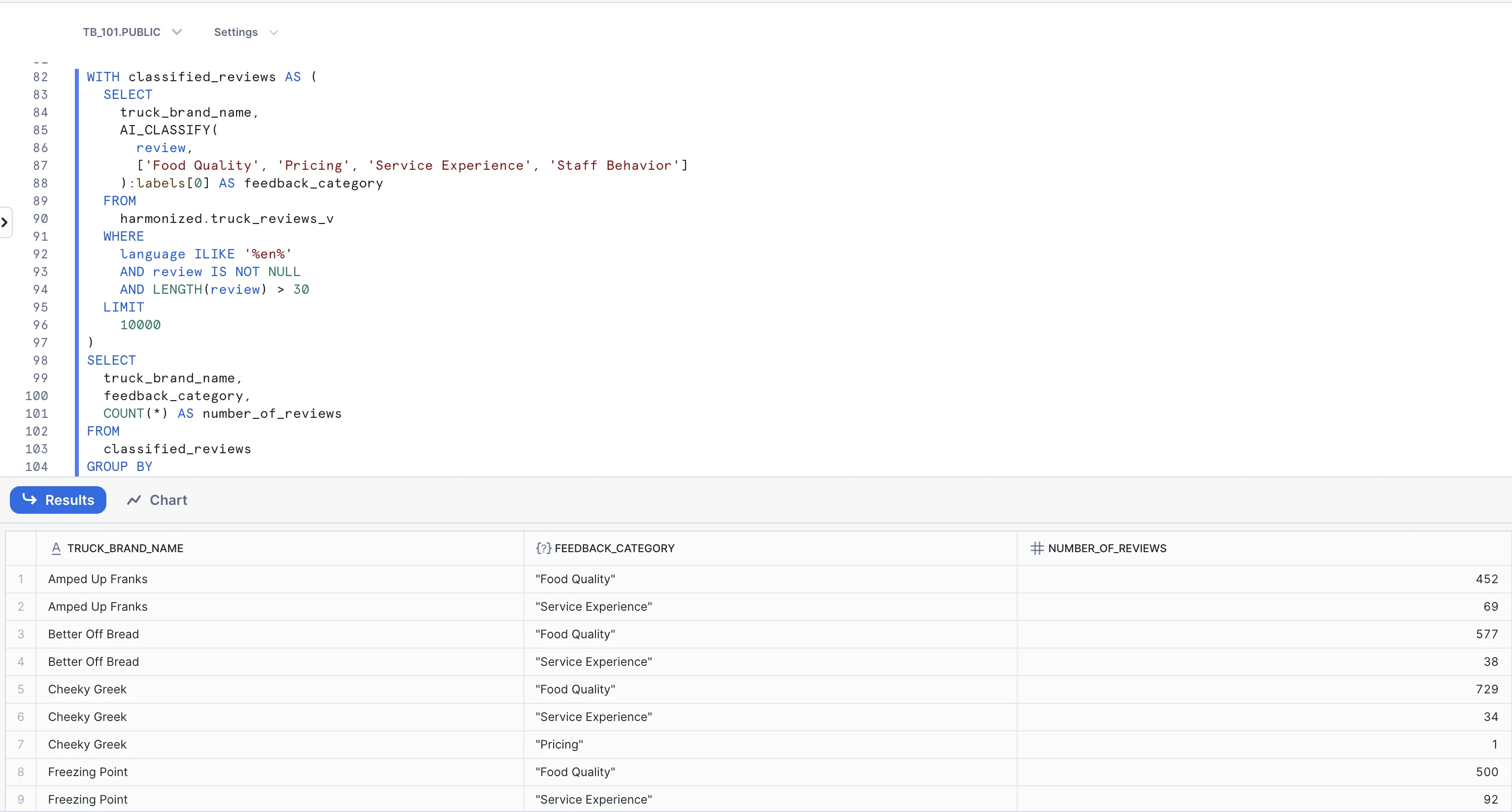

Step 4 - Extract Specific Insights
Key Insight
: Observe how
AI_CLASSIFY()
automatically categorized thousands of reviews into business-relevant themes
such as Food Quality, Service Experience, and more. We can instantly see that Food Quality is the most discussed topic across
our truck brands, providing the operations team with clear, actionable insight into customer priorities.
Next, to gain precise answers from unstructured text, we'll utilize the
EXTRACT_ANSWER()
function. This powerful function enables us to ask
specific business questions about customer feedback and receive direct answers. In this step, our goal is to identify precise operational issues
mentioned in customer reviews, highlighting specific problems that require immediate attention.
Business question:
“What specific improvement or complaint is mentioned in this review?"
Let's execute the next query:
SELECT
SELECT
truck_brand_name,
truck_brand_name,
primary_city,
primary_city,
LEFT(review, 100) || '...' AS review_preview,
LEFT(review, 100) || '...' AS review_preview,
SNOWFLAKE.CORTEX.EXTRACT_ANSWER(
SNOWFLAKE.CORTEX.EXTRACT_ANSWER(
review,
review,
'What specific improvement or complaint is mentioned in this review?'
'What specific improvement or complaint is mentioned in this review?'
) AS specific_feedback
) AS specific_feedback
FROM
FROM
harmonized.truck_reviews_v
harmonized.truck_reviews_v
WHERE
WHERE
language = 'en'
language = 'en'
AND review IS NOT NULL
AND review IS NOT NULL
AND LENGTH(review) > 50
AND LENGTH(review) > 50
ORDER BY truck_brand_name, primary_city ASC
ORDER BY truck_brand_name, primary_city ASC
LIMIT 10000;
LIMIT 10000;
9/26/26, 12:02 PM
Zero to Snowflake
https://www.snowflake.com/en/developers/guides/zero-to-snowflake/
25/59
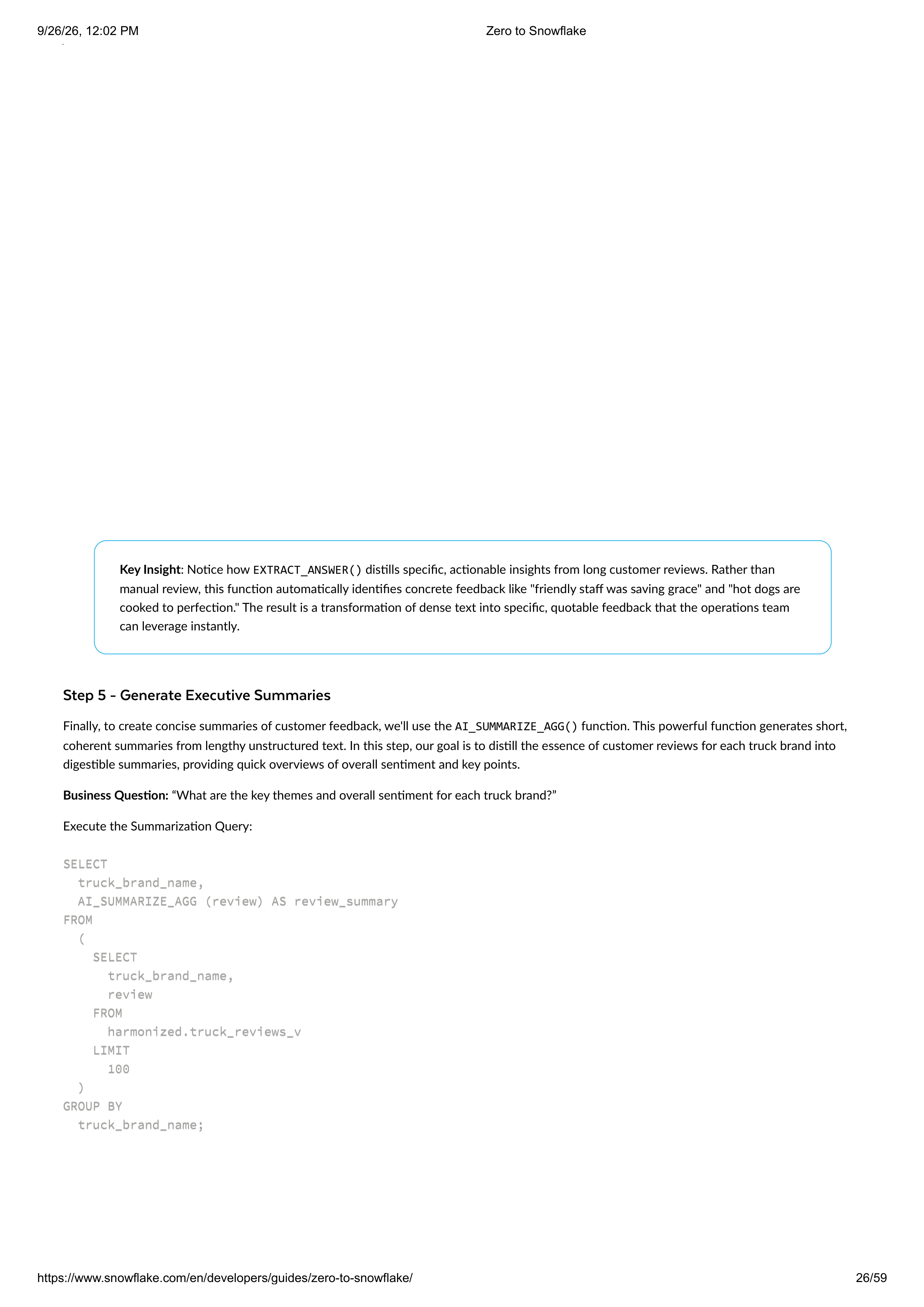


Step 5 - Generate Executive Summaries
Key Insight
: Notice how
EXTRACT_ANSWER()
distills specific, actionable insights from long customer reviews. Rather than
manual review, this function automatically identifies concrete feedback like "friendly staff was saving grace" and "hot dogs are
cooked to perfection." The result is a transformation of dense text into specific, quotable feedback that the operations team
can leverage instantly.
Finally, to create concise summaries of customer feedback, we'll use the
AI_SUMMARIZE_AGG()
function. This powerful function generates short,
coherent summaries from lengthy unstructured text. In this step, our goal is to distill the essence of customer reviews for each truck brand into
digestible summaries, providing quick overviews of overall sentiment and key points.
Business Question:
“What are the key themes and overall sentiment for each truck brand?”
Execute the Summarization Query:
SELECT
SELECT
truck_brand_name,
truck_brand_name,
AI_SUMMARIZE_AGG (review) AS review_summary
AI_SUMMARIZE_AGG (review) AS review_summary
FROM
FROM
(
(
SELECT
SELECT
truck_brand_name,
truck_brand_name,
review
review
FROM
FROM
harmonized.truck_reviews_v
harmonized.truck_reviews_v
LIMIT
LIMIT
100
100
)
)
GROUP BY
GROUP BY
truck_brand_name;
truck_brand_name;
9/26/26, 12:02 PM
Zero to Snowflake
https://www.snowflake.com/en/developers/guides/zero-to-snowflake/
26/59



Conclusion
Optional: Cortex Search
Overview
Step 1 - Access Cortex Search
Key Insight
: The
AI_SUMMARIZE_AGG()
function condenses lengthy reviews into clear, brand-level summaries. These
summaries highlight recurring themes and sentiment trends, providing decision-makers with quick overviews of each food
truck's performance and enabling faster understanding of customer perception without reading individual reviews.
We've successfully demonstrated the transformative power of AI Functions, shifting customer feedback analysis from individual review processing
to systemic, production-scale intelligence. Our journey through these four core functions clearly illustrates how each serves a distinct analytical
purpose, transforming raw customer voices into comprehensive business intelligence—systematic, scalable, and immediately actionable. What once
required individual review analysis now processes thousands of reviews in seconds, providing both the emotional context and specific details
crucial for data-driven operational improvements.
While AI-powered tools excel at generating complex analytical queries, a common daily challenge for customer service teams is quickly finding
specific customer reviews for complaints or compliments. Traditional keyword search often falls short, missing the nuances of natural language.
Snowflake Cortex Search
solves this by providing low-latency, high-quality "fuzzy" search over your Snowflake text data. It quickly sets up hybrid
(vector and keyword) search engines, handling embeddings, infrastructure, and tuning for you. Under the hood, Cortex Search combines semantic
(meaning-based) and lexical (keyword-based) retrieval with intelligent re-ranking to deliver the most relevant results. In this lab, you will configure a
search service, connect it to customer review data, and run semantic queries to proactively identify key customer feedback.
1. Open Snowsight and navigate to the AI & ML Studio, then select
Cortex Search
.
2. Click
Create
to begin setup.
This opens the search service configuration interface, where you’ll define how Snowflake indexes and interprets your text data.
9/26/26, 12:02 PM
Zero to Snowflake
https://www.snowflake.com/en/developers/guides/zero-to-snowflake/
27/59

Step 2 - Configure the Search Service
Step 3 - Connect to Review Data
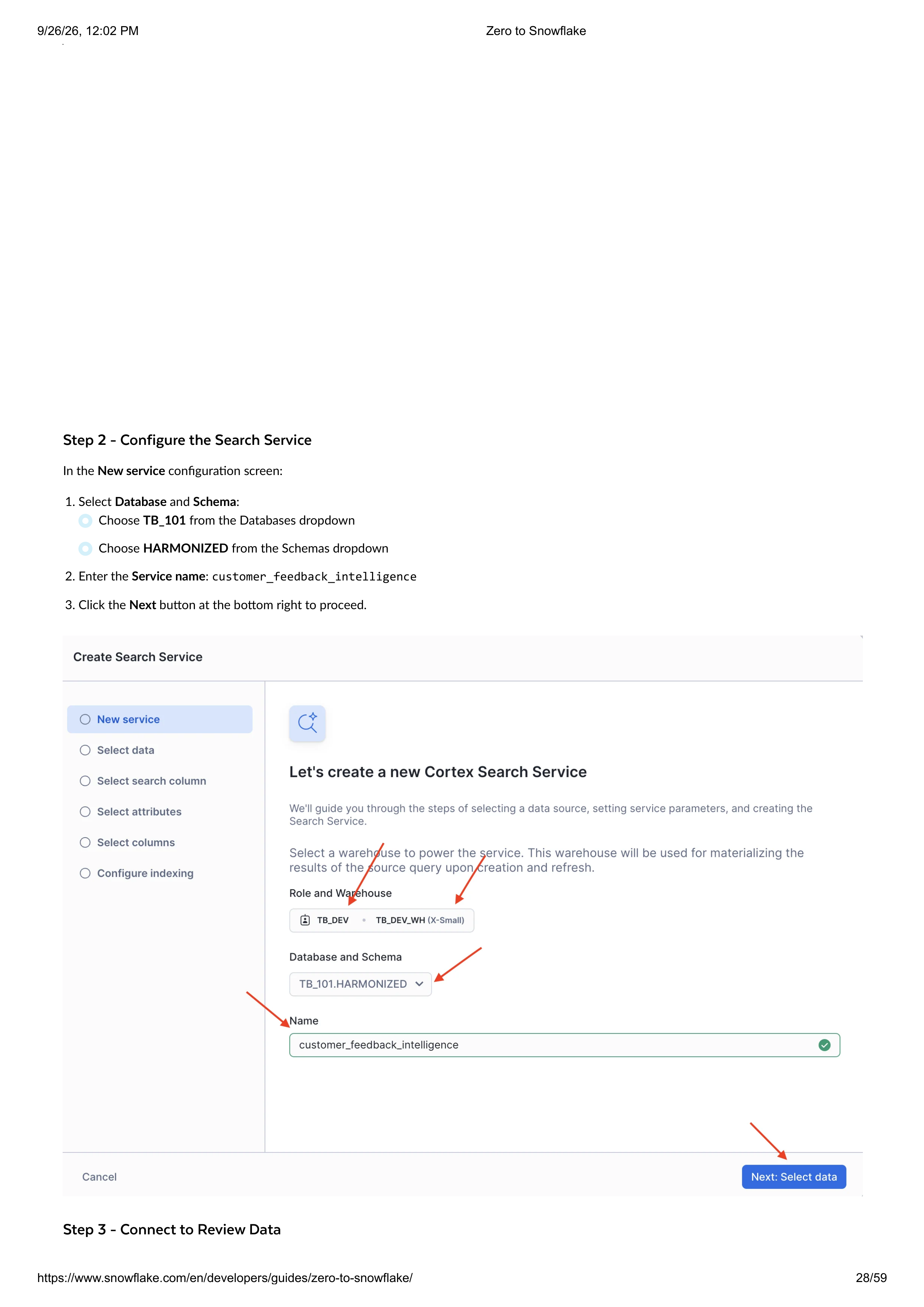
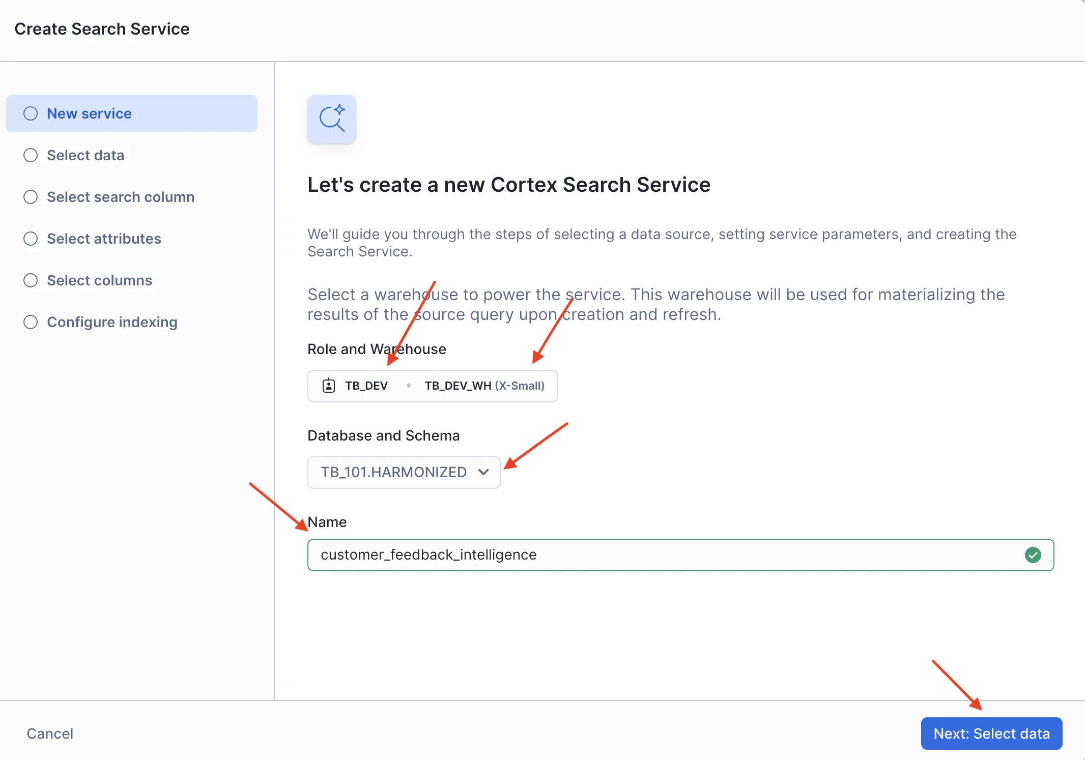
In the
New service
configuration screen:
1. Select
Database
and
Schema
:
2. Enter the
Service name
:
customer_feedback_intelligence
3. Click the
Next
button at the bottom right to proceed.
Choose
TB_101
from the Databases dropdown
Choose
HARMONIZED
from the Schemas dropdown
9/26/26, 12:02 PM
Zero to Snowflake
https://www.snowflake.com/en/developers/guides/zero-to-snowflake/
28/59
The wizard will now guide you through several configuration screens. Follow these steps:
1.
2.
3.
4.
5.
Select data screen:
From the Views dropdown, select
TRUCK_REVIEWS_V
Click
Next
Select search column screen:
Choose
REVIEW
(this is the text column that will be semantically searched)
Click
Next
Select attributes screen:
Select columns for filtering results:
TRUCK_BRAND_NAME
,
PRIMARY_CITY
,
REVIEW_ID
Click
Next
Select columns screen:
Choose other columns to include in search results such as
DATE
,
LANGUAGE
, etc.
Click
Next
Configure indexing screen:
Warehouse
: Select
COMPUTE_WH
from the dropdown
Accept the other default settings
Click
Create
to build the search service
Note
: Creating the search service includes building the index, so the initial setup may take a little longer. If the creation
process is taking an extended period, you can seamlessly continue the lab by using a pre-configured search service:
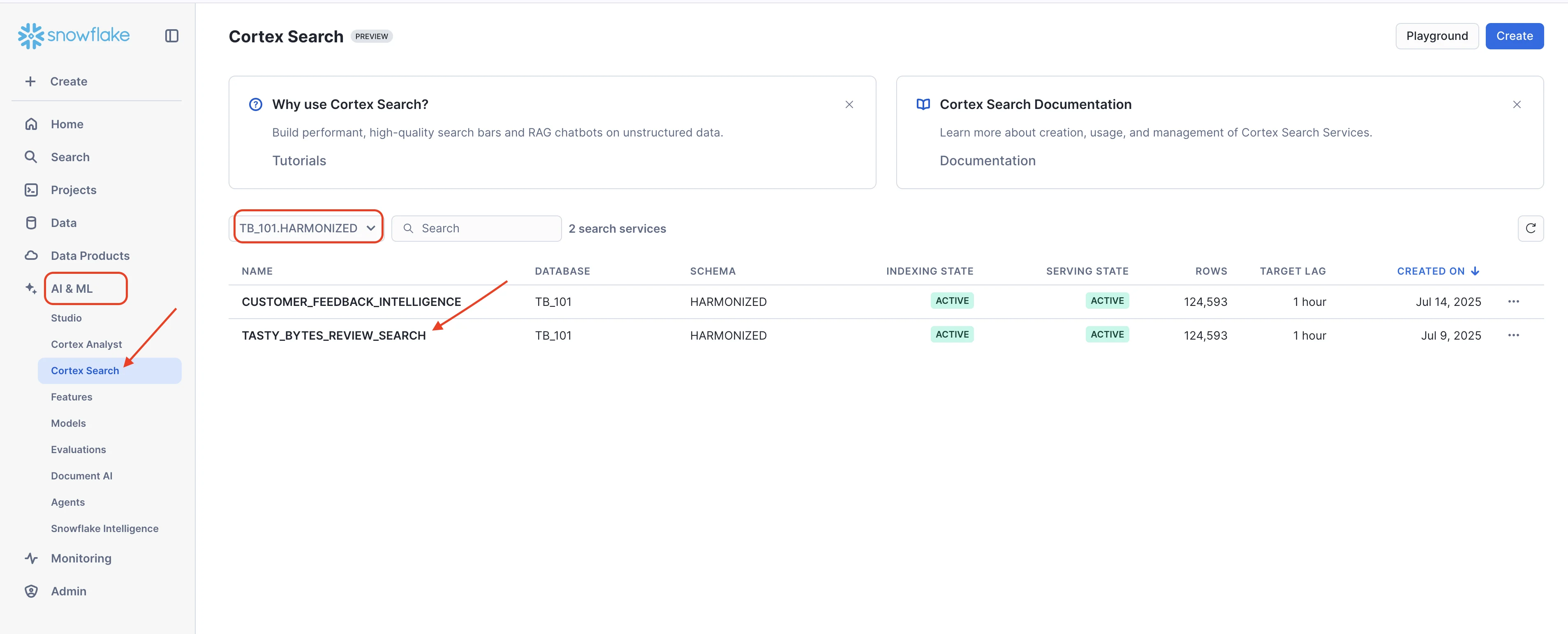
1. From the left-hand menu in Snowsight, navigate to
AI & ML
, then click on
Cortex Search
.
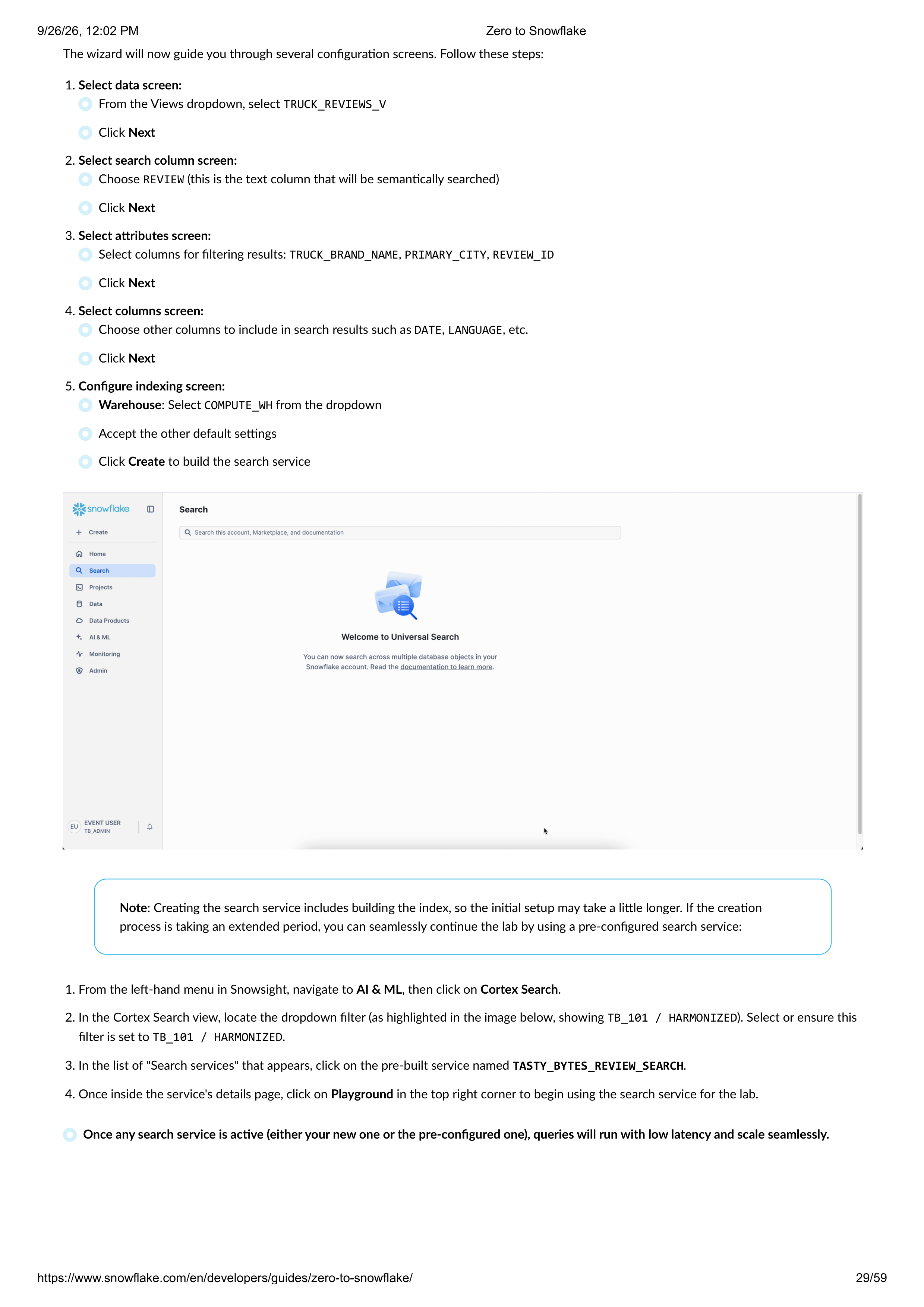
2. In the Cortex Search view, locate the dropdown filter (as highlighted in the image below, showing
TB_101 / HARMONIZED
). Select or ensure this
filter is set to
TB_101 / HARMONIZED
.
3. In the list of "Search services" that appears, click on the pre-built service named
TASTY_BYTES_REVIEW_SEARCH
.
4. Once inside the service's details page, click on
Playground
in the top right corner to begin using the search service for the lab.
Once any search service is active (either your new one or the pre-configured one), queries will run with low latency and scale seamlessly.
9/26/26, 12:02 PM
Zero to Snowflake
https://www.snowflake.com/en/developers/guides/zero-to-snowflake/
29/59


Step 4 - Run Semantic Query
Behind this simple UI, Cortex Search is performing a complex task. It analyzes the text in your "REVIEW" column, using an AI
model to generate semantic embeddings, which are numerical representations of the text's meaning. These embeddings are
then indexed, allowing for high-speed conceptual searches later on. In just a few clicks, you have taught Snowflake to
understand the intent behind your reviews.
When the service shows as "Active", click on
Playground
and enter the natural language prompt in the search bar:
Prompt - 1:
Customers getting sick
Key Insight
: Notice Cortex Search isn’t just finding customers - it’s finding CONDITIONS that could MAKE customers sick.
That is the difference between reactive keyword search and proactive semantic understanding.
Now try another query:
Prompt - 2:
Angry customers
9/26/26, 12:02 PM
Zero to Snowflake
https://www.snowflake.com/en/developers/guides/zero-to-snowflake/
30/59


Conclusion
Optional: Cortex Analyst
Overview
Step 1 - Design Semantic Model
Key Insight
: These customers are about to churn, but they never said “I’m angry.” They expressed frustration in their own
words. Cortex Search understands the emotion behind the language, helping you identify and save at-risk customers before
they leave.
Ultimately, Cortex Search transforms how Tasty Bytes analyzes customer feedback. It empowers the customer service manager to move beyond
simply sifting through reviews, to truly understand and proactively act upon the voice of the customer at scale, driving better operational decisions
and enhancing customer loyalty.
In the next module - Cortex Analyst - you'll use natural language to query structured data.
A business analyst at Tasty Bytes needs to enable self-service analytics, allowing the business team to ask complex questions in natural language
and get instant insights without relying on data analysts to write SQL. While previous AI tools helped with finding reviews and complex query
generation, the demand now is for
conversational analytics
that directly transforms structured business data into immediate insights.
Snowflake Cortex Analyst
empowers business users to ask sophisticated questions directly, seamlessly extracting value from their analytics data
through natural language interaction. This lab will guide you through designing a semantic model, connecting it to your business data, configuring
relationships and synonyms, and then executing advanced business intelligence queries using natural language.
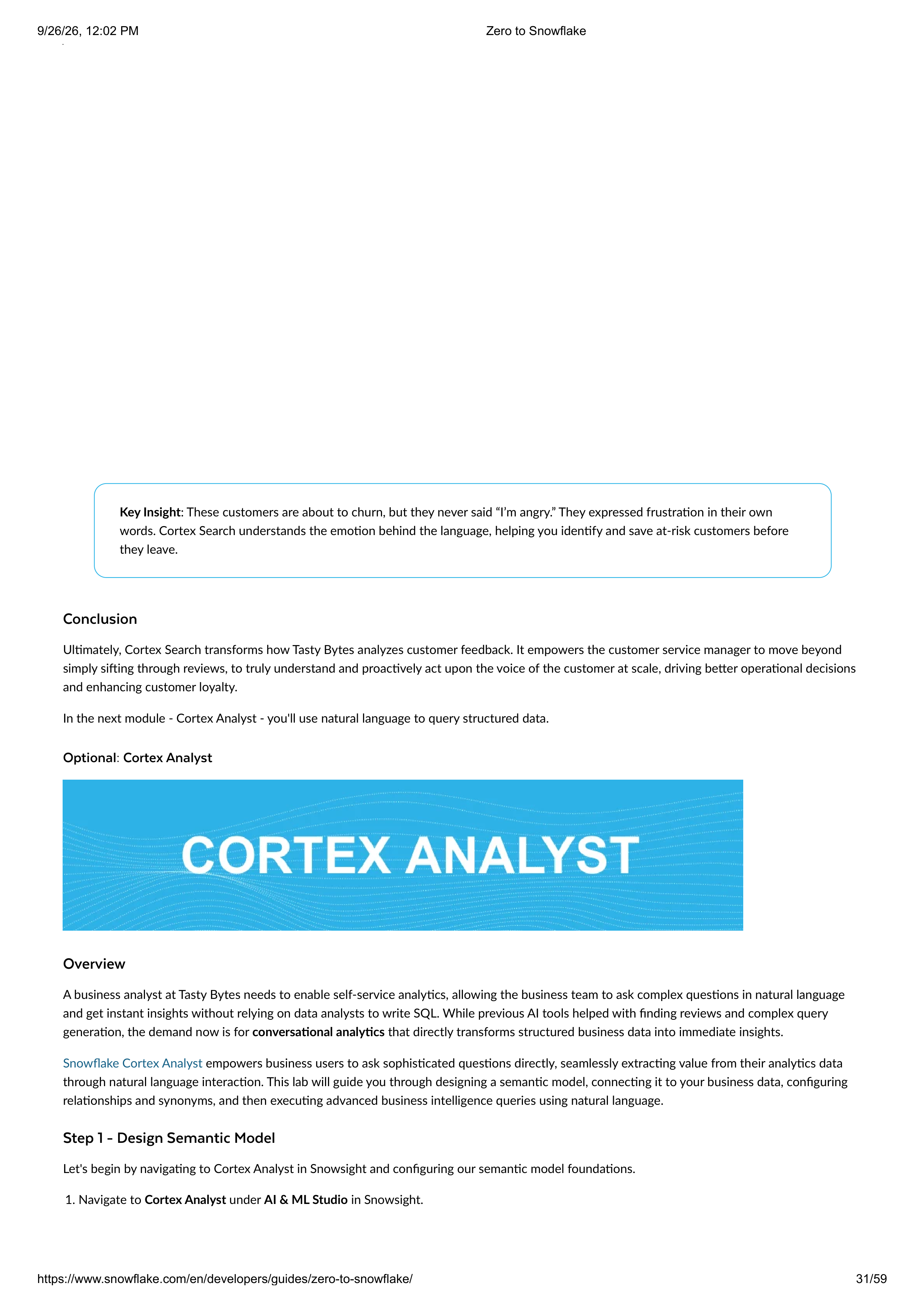
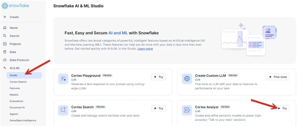
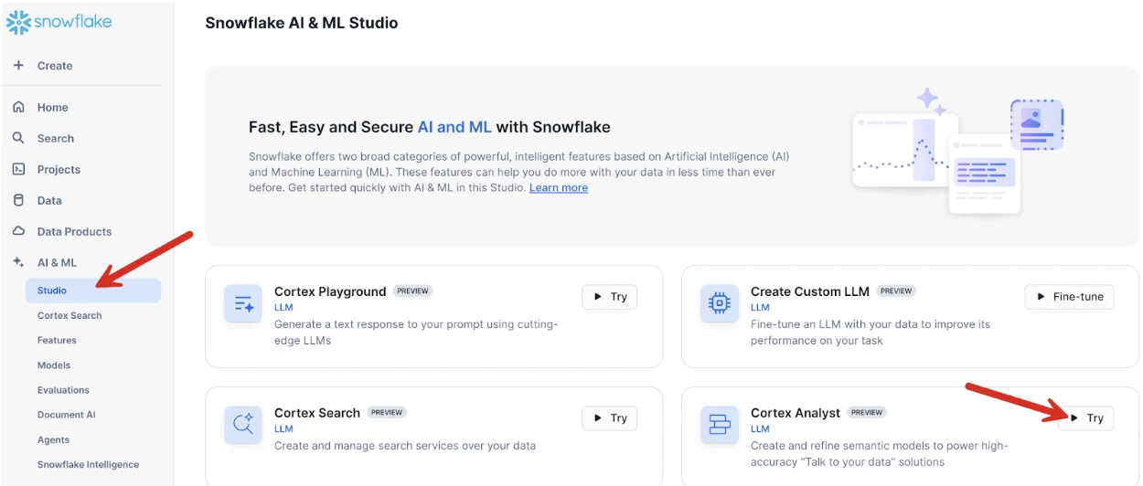
Let's begin by navigating to Cortex Analyst in Snowsight and configuring our semantic model foundations.
1. Navigate to
Cortex Analyst
under
AI & ML Studio
in Snowsight.
9/26/26, 12:02 PM
Zero to Snowflake
https://www.snowflake.com/en/developers/guides/zero-to-snowflake/
31/59
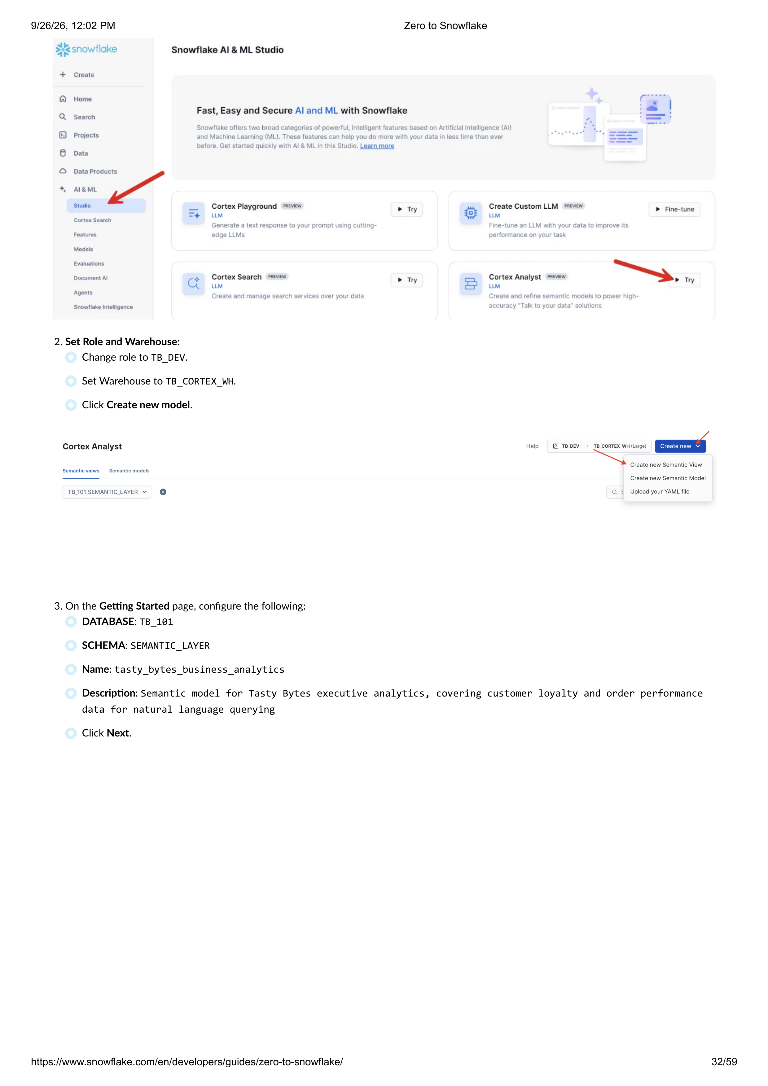
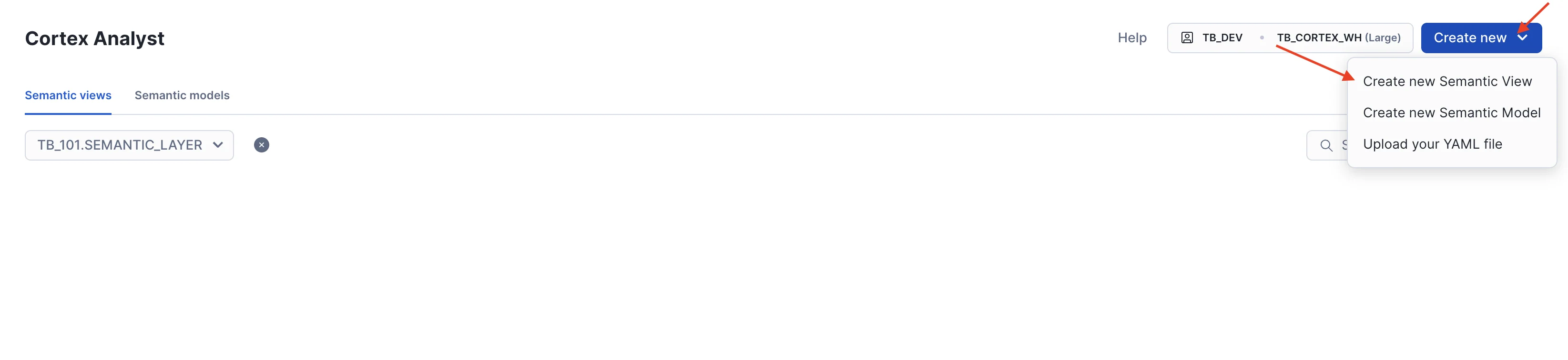
2.
Set Role and Warehouse:
Change role to
TB_DEV
.
Set Warehouse to
TB_CORTEX_WH
.
Click
Create new model
.
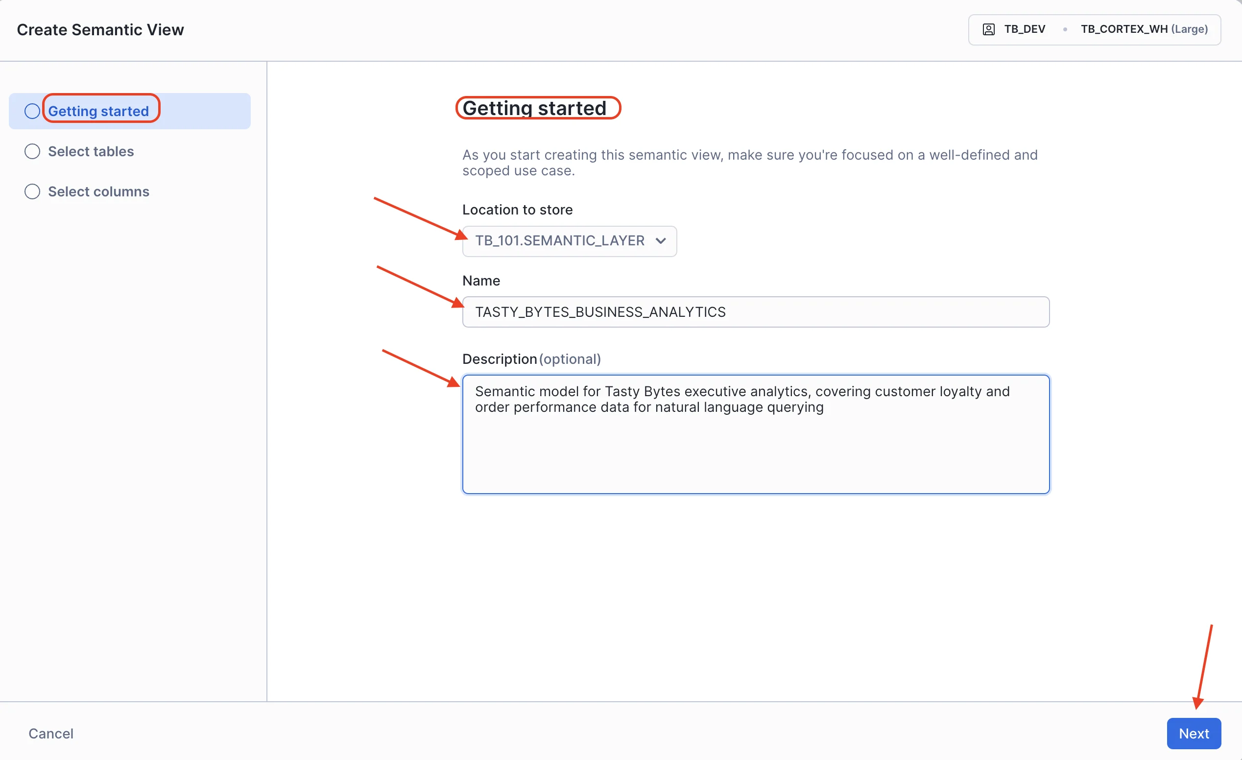
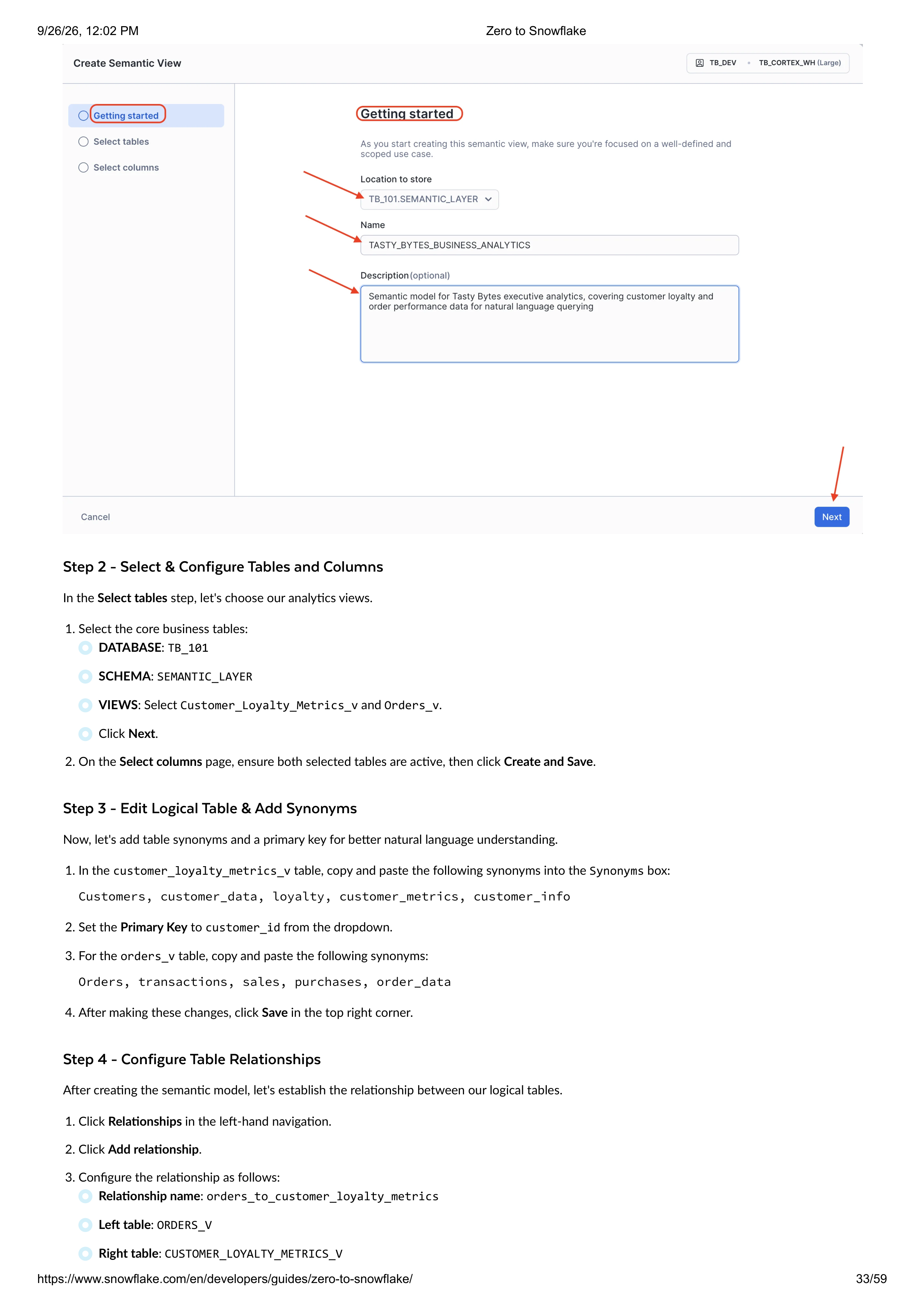
3. On the
Getting Started
page, configure the following:
DATABASE
:
TB_101
SCHEMA
:
SEMANTIC_LAYER
Name
:
tasty_bytes_business_analytics
Description
:
Semantic model for Tasty Bytes executive analytics, covering customer loyalty and order performance
data for natural language querying
Click
Next
.
9/26/26, 12:02 PM
Zero to Snowflake
https://www.snowflake.com/en/developers/guides/zero-to-snowflake/
32/59
Step 2 - Select & Configure Tables and Columns
Step 3 - Edit Logical Table & Add Synonyms
Step 4 - Configure Table Relationships
In the
Select tables
step, let's choose our analytics views.
1.
2.
Select the core business tables:
DATABASE
:
TB_101
SCHEMA
:
SEMANTIC_LAYER
VIEWS
: Select
Customer_Loyalty_Metrics_v
and
Orders_v
.
Click
Next
.
On the
Select columns
page, ensure both selected tables are active, then click
Create and Save
.
Now, let's add table synonyms and a primary key for better natural language understanding.
1.
2.
3.
4.
In the
customer_loyalty_metrics_v
table, copy and paste the following synonyms into the
Synonyms
box:
Customers, customer_data, loyalty, customer_metrics, customer_info
Set the
Primary Key
to
customer_id
from the dropdown.
For the
orders_v
table, copy and paste the following synonyms:
Orders, transactions, sales, purchases, order_data
After making these changes, click
Save
in the top right corner.
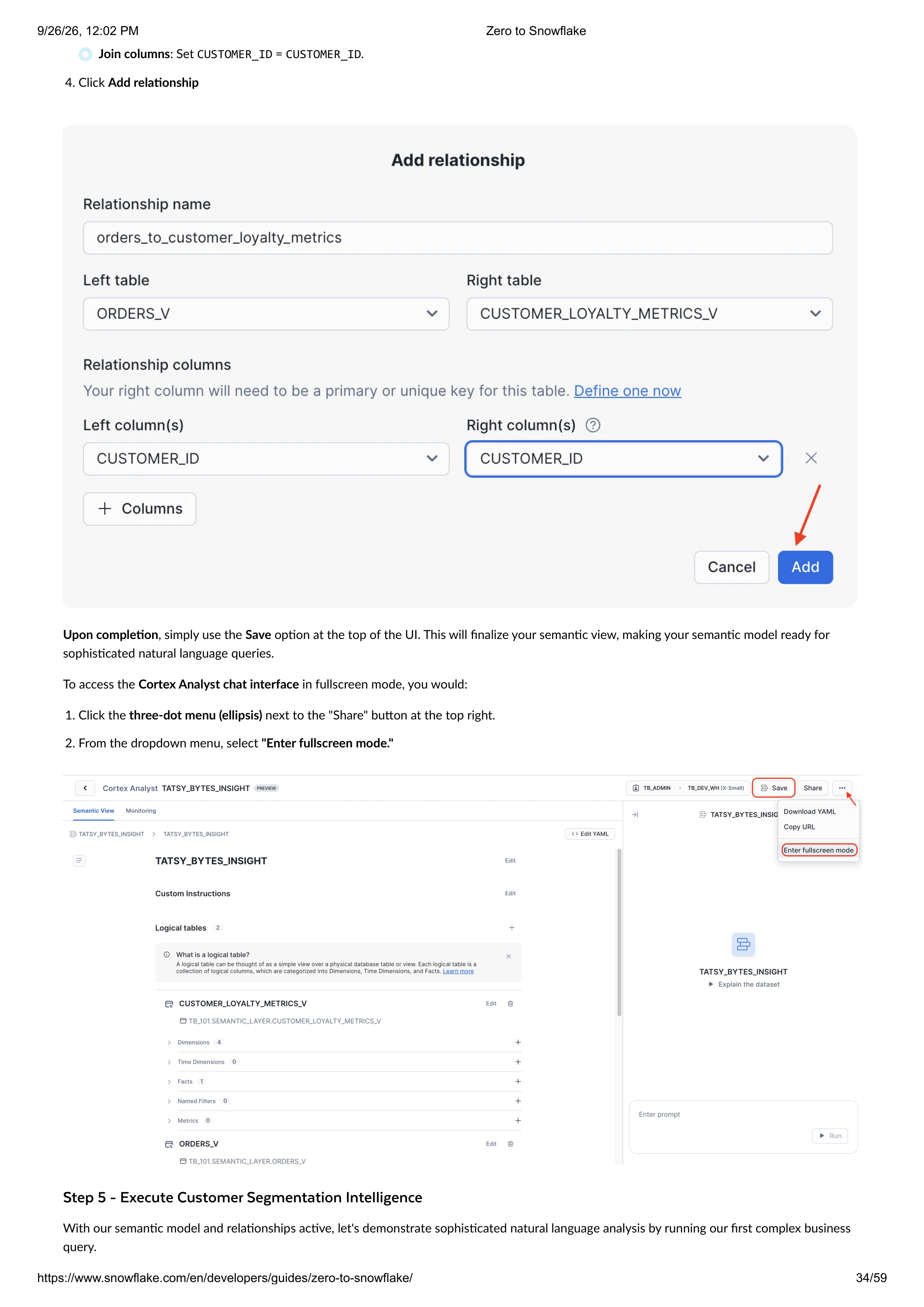
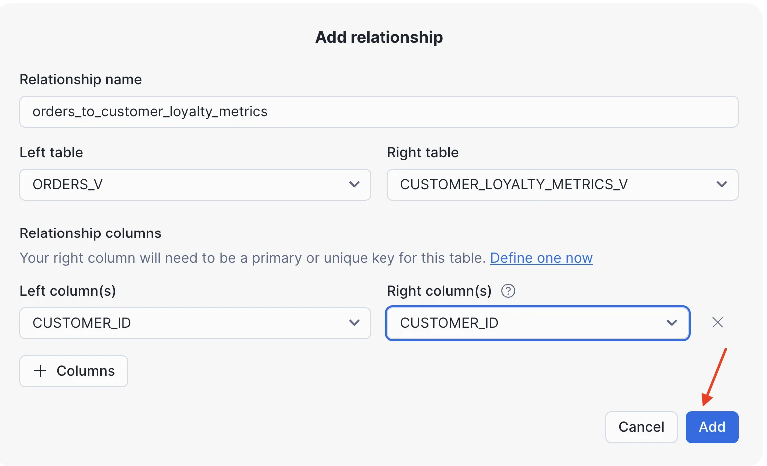
After creating the semantic model, let's establish the relationship between our logical tables.
1.
2.
3.
Click
Relationships
in the left-hand navigation.
Click
Add relationship
.
Configure the relationship as follows:
Relationship name
:
orders_to_customer_loyalty_metrics
Left table
:
ORDERS_V
Right table
:
CUSTOMER_LOYALTY_METRICS_V
9/26/26, 12:02 PM
Zero to Snowflake
https://www.snowflake.com/en/developers/guides/zero-to-snowflake/
33/59
Step 5 - Execute Customer Segmentation Intelligence
4.
Join columns
: Set
CUSTOMER_ID
=
CUSTOMER_ID
.
Click
Add relationship
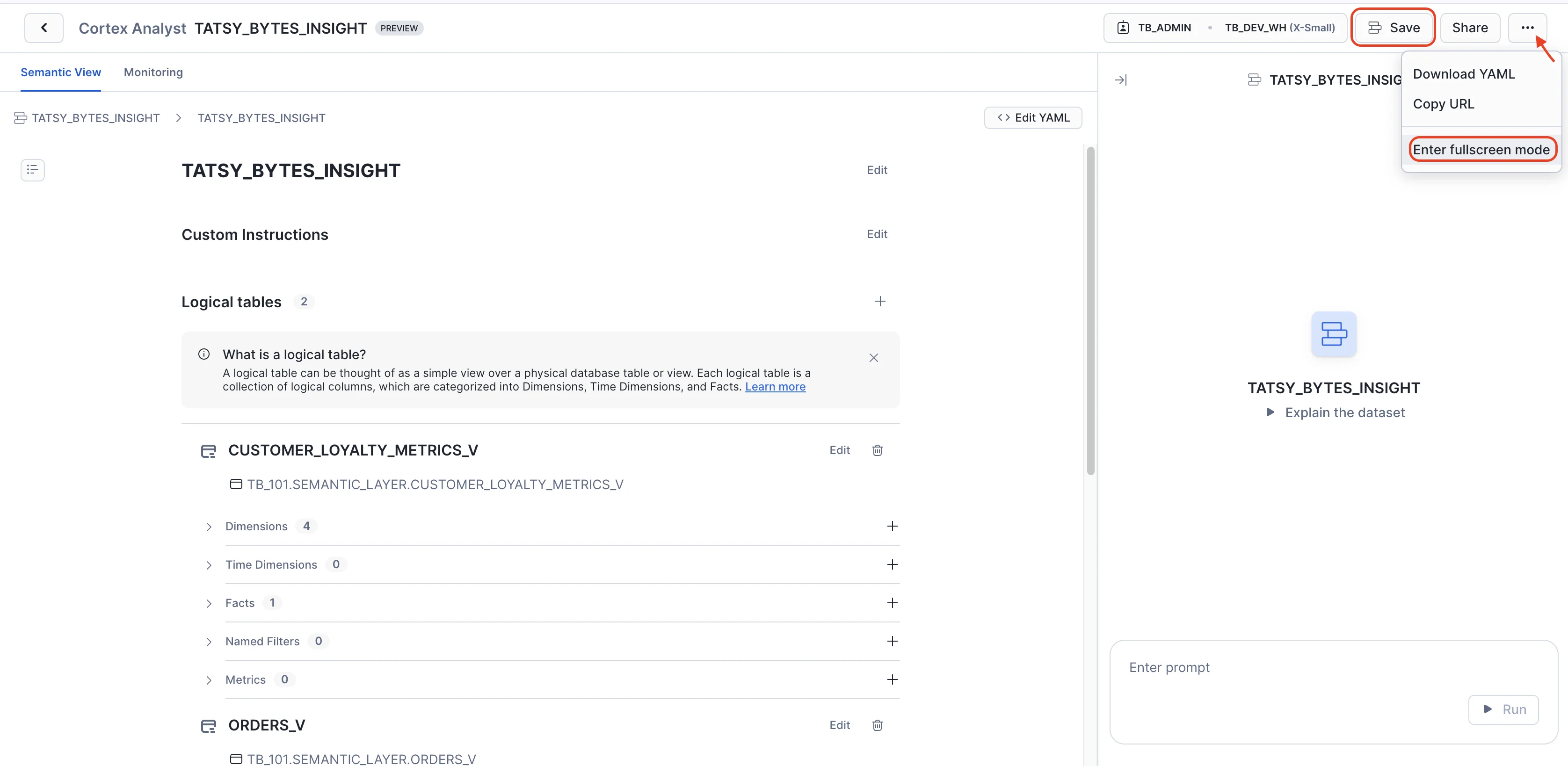
Upon completion
, simply use the
Save
option at the top of the UI. This will finalize your semantic view, making your semantic model ready for
sophisticated natural language queries.
To access the
Cortex Analyst chat interface
in fullscreen mode, you would:
1. Click the
three-dot menu (ellipsis)
next to the "Share" button at the top right.
2. From the dropdown menu, select
"Enter fullscreen mode."
With our semantic model and relationships active, let's demonstrate sophisticated natural language analysis by running our first complex business
query.
9/26/26, 12:02 PM
Zero to Snowflake
https://www.snowflake.com/en/developers/guides/zero-to-snowflake/
34/59


Step 6 - Generate Advanced Business Intelligence
1.
2.
Navigate to the Cortex Analyst query interface.
Enter the following prompt:
Show customer groups by marital status and gender, with their total spending per customer and average order
Key Insight
: Instantly delivers comprehensive intelligence by combining multi-table joins, demographic segmentation,
geographic insights, and lifetime value analysis - insights that would require 40+ lines of SQL and hours of analyst effort.
Having seen basic segmentation, let's now demonstrate enterprise-grade SQL that showcases the full power of conversational business
intelligence.
1.
2.
Clear the context by clicking the refresh icon.
Enter the following prompt:
I want to understand our customer base better. Can you group customers by their total spending (high, medium
9/26/26, 12:02 PM
Zero to Snowflake
https://www.snowflake.com/en/developers/guides/zero-to-snowflake/
35/59


Conclusion
Snowflake CoWork
Overview
Key Insight
: Notice how Cortex Analyst seamlessly bridges the gap between a business user's simple, natural language
question and the sophisticated, multi-faceted SQL query required to answer it. It automatically constructs the complex logic,
including CTEs, window functions, and detailed aggregations, that would typically demand a skilled data analyst.
Through these rigorous steps, we've forged a robust Cortex Analyst semantic model. This isn't just an improvement; it's a transformative tool
designed to liberate users across various industries from the constraints of SQL, enabling them to surface profound business intelligence through
intuitive natural language queries. Our multi-layered analyses, while showcased through the Tasty Bytes use case, powerfully illustrate how this
model drastically cuts down on the time and effort traditionally needed for deep insights, thereby democratizing access to data and fueling a
culture of informed, agile decision-making on a broad scale.
The Chief Operating Officer at Tasty Bytes receives dozens of fragmented reports each week: customer satisfaction dashboards, revenue analytics,
operational performance metrics, and market analysis. Critical business insights remain buried across separate systems: customer sentiment lives in
review platforms, sales data sits in financial dashboards, and operational metrics exist in isolated performance tools.
When the COO needs to understand why Q3 revenue dropped, connecting customer feedback sentiment with actual financial performance
requires hours of manual analysis, SQL expertise, and cross-referencing multiple data sources. This is a significant hurdle for executives and other
non-technical roles.
In this section, we'll demonstrate how
Snowflake CoWork
tackles this challenge by combining the capabilities of Cortex Search and Cortex Analyst,
which are made available through the setup. This integration allows for a single conversational AI agent. You'll see how executives and other non-
technical roles can ask natural language questions and receive immediate answers with visualizations. This kind of insight would normally take
weeks of analyst work across multiple teams.
Prerequisites:
9/26/26, 12:02 PM
Zero to Snowflake
https://www.snowflake.com/en/developers/guides/zero-to-snowflake/
36/59
Step 1 - Upload Semantic Model
Step 2: Create a Unified Agent
Before starting this module, your environment includes pre-configured AI services that power Snowflake CoWork:
Cortex Search Service:
tasty_bytes_review_search
- analyzing customer reviews and feedback
Note for Advanced Users: If you want to build your own Cortex Search from scratch, an optional setup module is available. For a detailed
guide, click the link to the:
Cortex Search Module
Cortex Analyst Service:
TASTY_BYTES_BUSINESS_ANALYTICS
- for translating natural language questions into SQL and providing insights from
structured data, enabling self-service analytics.
Note for Advanced Users: If you prefer to build your own Cortex Analyst semantic model from scratch, you can access the detailed setup
module for guidance. Access the detailed setup by clicking on the:
Cortex Analyst Module
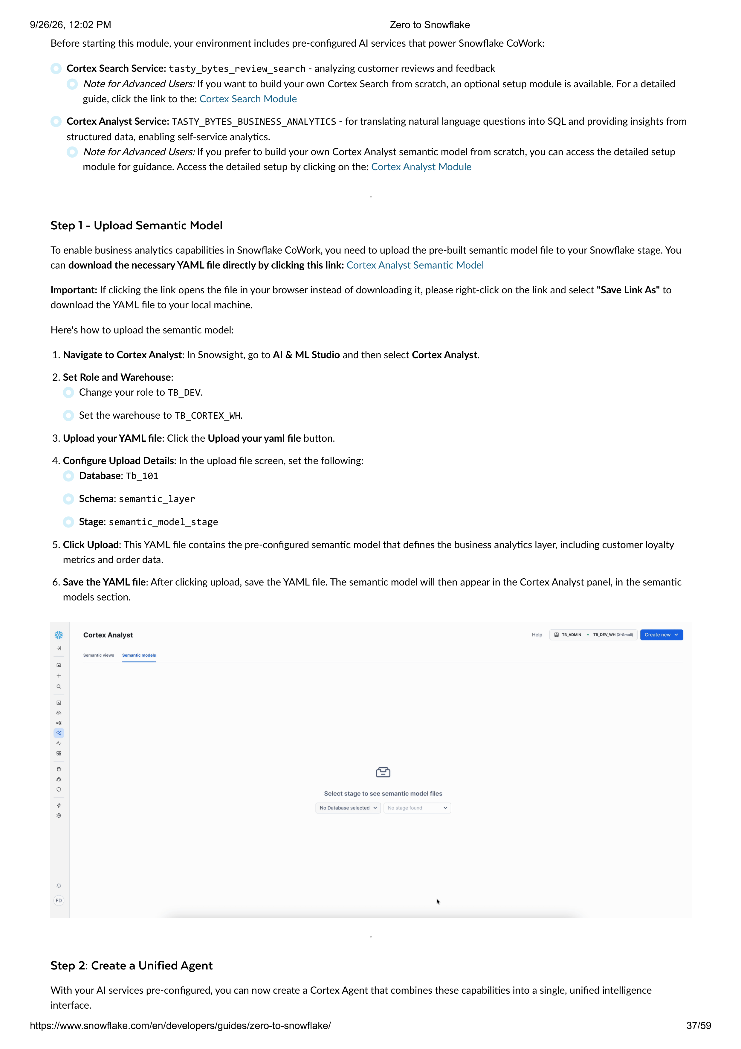
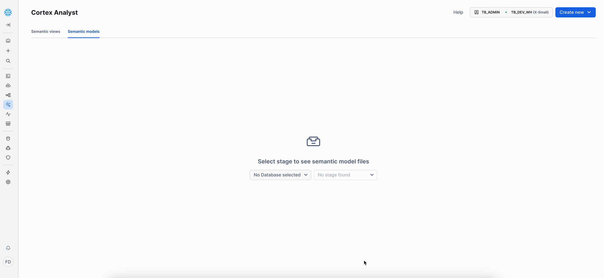
To enable business analytics capabilities in Snowflake CoWork, you need to upload the pre-built semantic model file to your Snowflake stage. You
can
download the necessary YAML file directly by clicking this link:
Cortex Analyst Semantic Model
Important:
If clicking the link opens the file in your browser instead of downloading it, please right-click on the link and select
"Save Link As"
to
download the YAML file to your local machine.
Here's how to upload the semantic model:
1.
2.
3.
4.
5.
6.
Navigate to Cortex Analyst
: In Snowsight, go to
AI & ML Studio
and then select
Cortex Analyst
.
Set Role and Warehouse
:
Change your role to
TB_DEV
.
Set the warehouse to
TB_CORTEX_WH
.
Upload your YAML file
: Click the
Upload your yaml file
button.
Configure Upload Details
: In the upload file screen, set the following:
Database
:
Tb_101
Schema
:
semantic_layer
Stage
:
semantic_model_stage
Click Upload
: This YAML file contains the pre-configured semantic model that defines the business analytics layer, including customer loyalty
metrics and order data.
Save the YAML file
: After clicking upload, save the YAML file. The semantic model will then appear in the Cortex Analyst panel, in the semantic
models section.
With your AI services pre-configured, you can now create a Cortex Agent that combines these capabilities into a single, unified intelligence
interface.
9/26/26, 12:02 PM
Zero to Snowflake
https://www.snowflake.com/en/developers/guides/zero-to-snowflake/
37/59
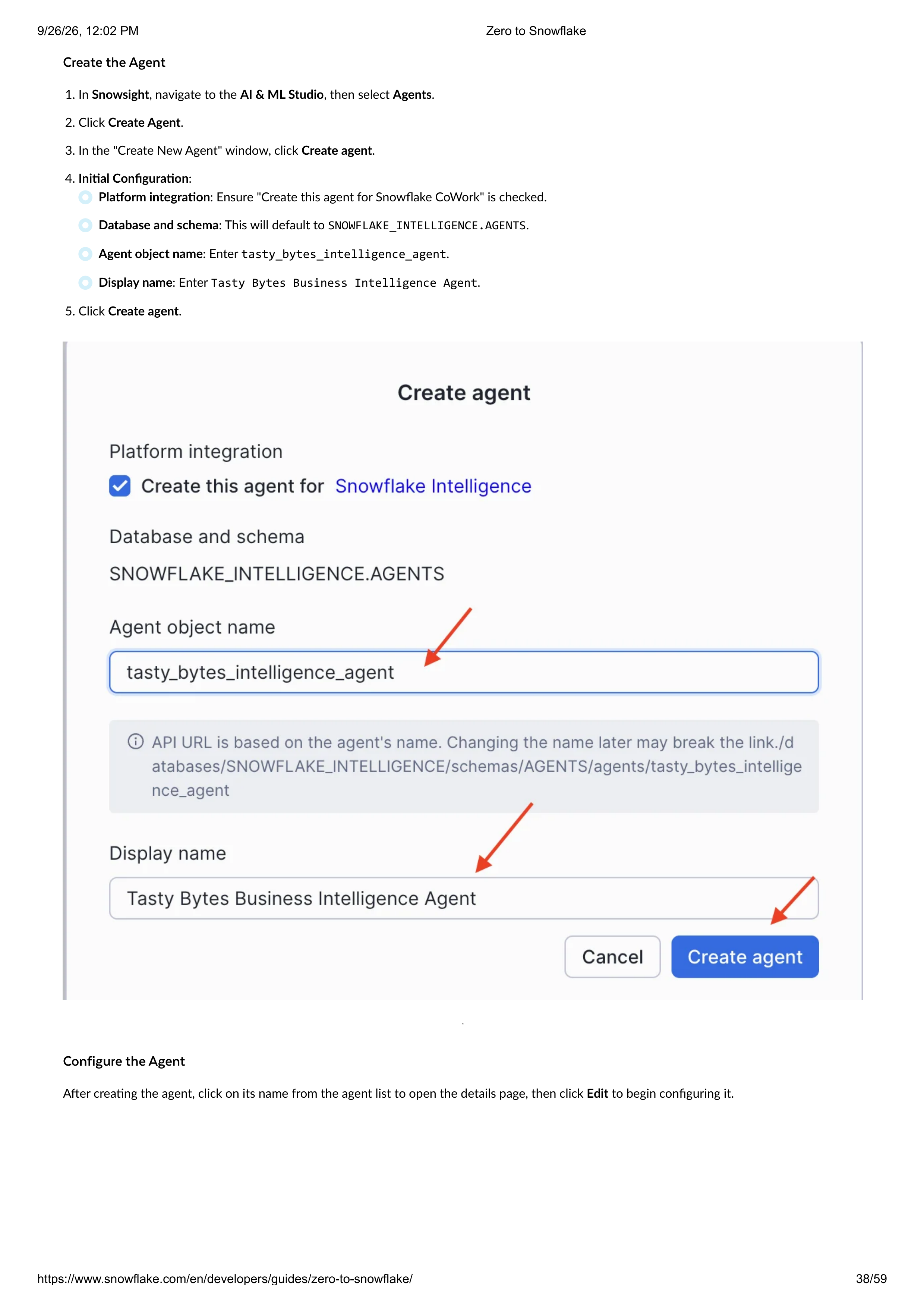
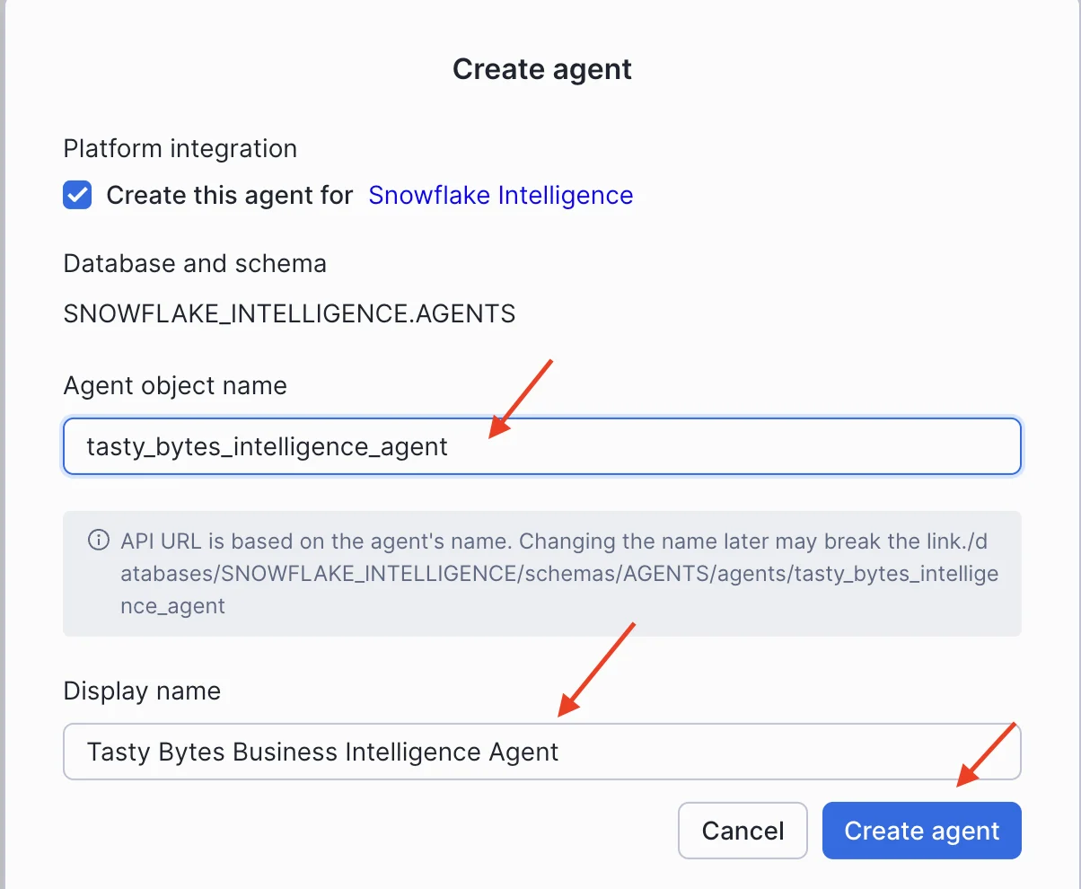
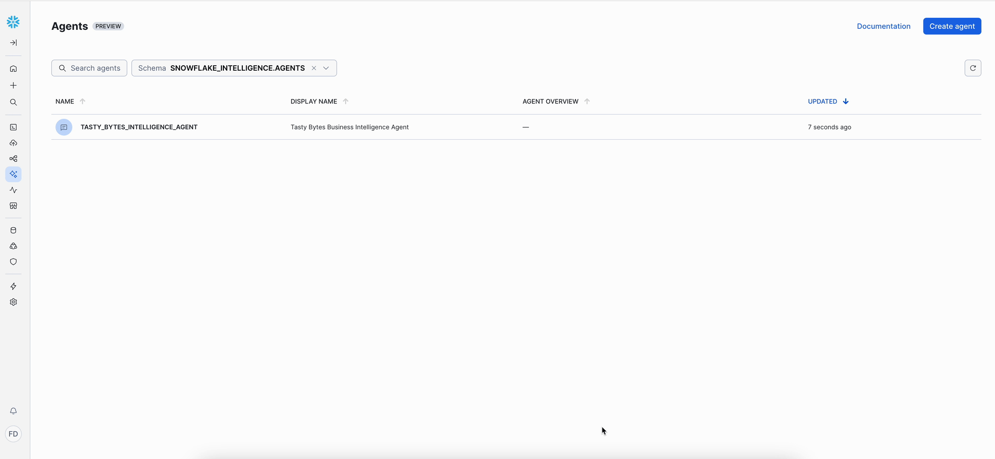
Create the Agent
Configure the Agent
1. In
Snowsight
, navigate to the
AI & ML Studio
, then select
Agents
.
2. Click
Create Agent
.
3. In the "Create New Agent" window, click
Create agent
.
4.
Initial Configuration
:
5. Click
Create agent
.
Platform integration
: Ensure "Create this agent for Snowflake CoWork" is checked.
Database and schema
: This will default to
SNOWFLAKE_INTELLIGENCE.AGENTS
.
Agent object name
: Enter
tasty_bytes_intelligence_agent
.
Display name
: Enter
Tasty Bytes Business Intelligence Agent
.
After creating the agent, click on its name from the agent list to open the details page, then click
Edit
to begin configuring it.
9/26/26, 12:02 PM
Zero to Snowflake
https://www.snowflake.com/en/developers/guides/zero-to-snowflake/
38/59
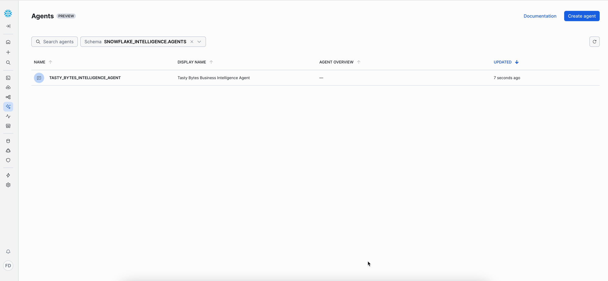
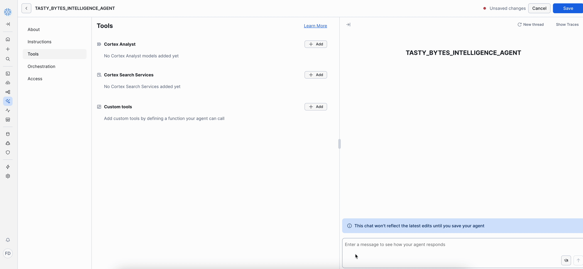
1. About Tab
2. Tools Tab
Display name
:
Tasty Bytes Business Intelligence Agent
Description
:
This agent analyzes customer feedback and business performance data for Tasty Bytes food trucks. It identifies
Note
: This lab primarily uses a pre-built
semantic model
uploaded in Step 1. However, if you built your Cortex Analyst
semantic view from scratch using the
Cortex Analyst Module
, you will select your
semantic view
here instead of a semantic
model. After setting the
Database
to
TB_101
and
Schema
to
semantic_layer
, your semantic view will be listed and
selectable under that schema.
Now, let's add the semantic model we uploaded in Step 1:
Add the Cortex Analyst Tool:
1. Click
Add
next to "Cortex Analyst."
2. Select the
Semantic model file
radio button.
3.
Configure the semantic model location
:
4.
Configure tool details
:
Schema
: Choose
TB_101.SEMANTIC_LAYER
.
Stage
: Choose
SEMANTIC_MODEL_STAGE
.
File Selection
: Pick your uploaded YAML file from the list.
Name
: Enter
tasty_bytes_business_analytics
.
Description
:
Searches customer reviews and feedback to identify sentiment, operational issues, and customer satisfaction in
5.
Configure execution settings
:
6. Click
Add
.
Warehouse
: Select
Custom
and choose
TB_CORTEX_WH
.
Query timeout
: Enter
300
.
9/26/26, 12:02 PM
Zero to Snowflake
https://www.snowflake.com/en/developers/guides/zero-to-snowflake/
39/59
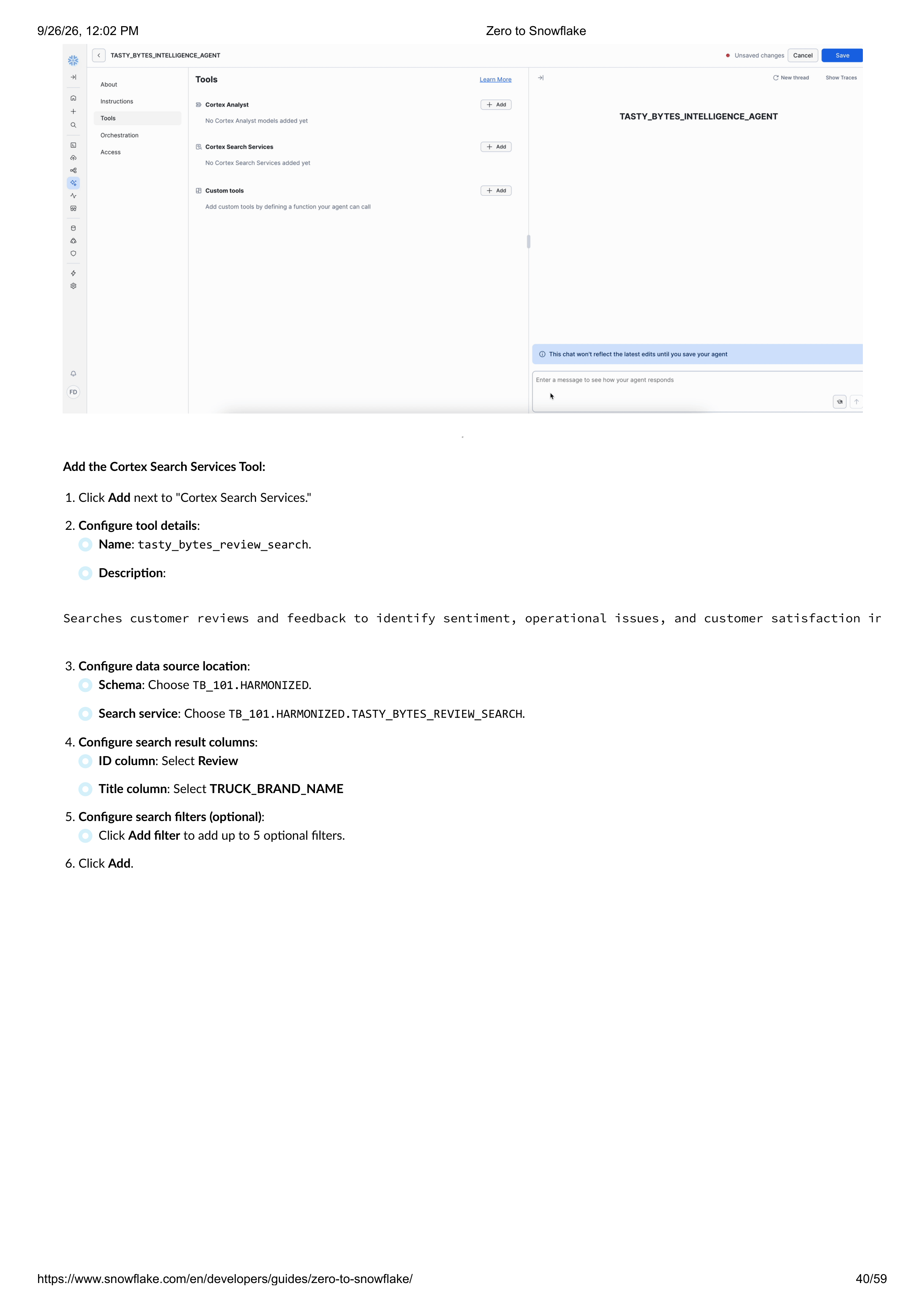
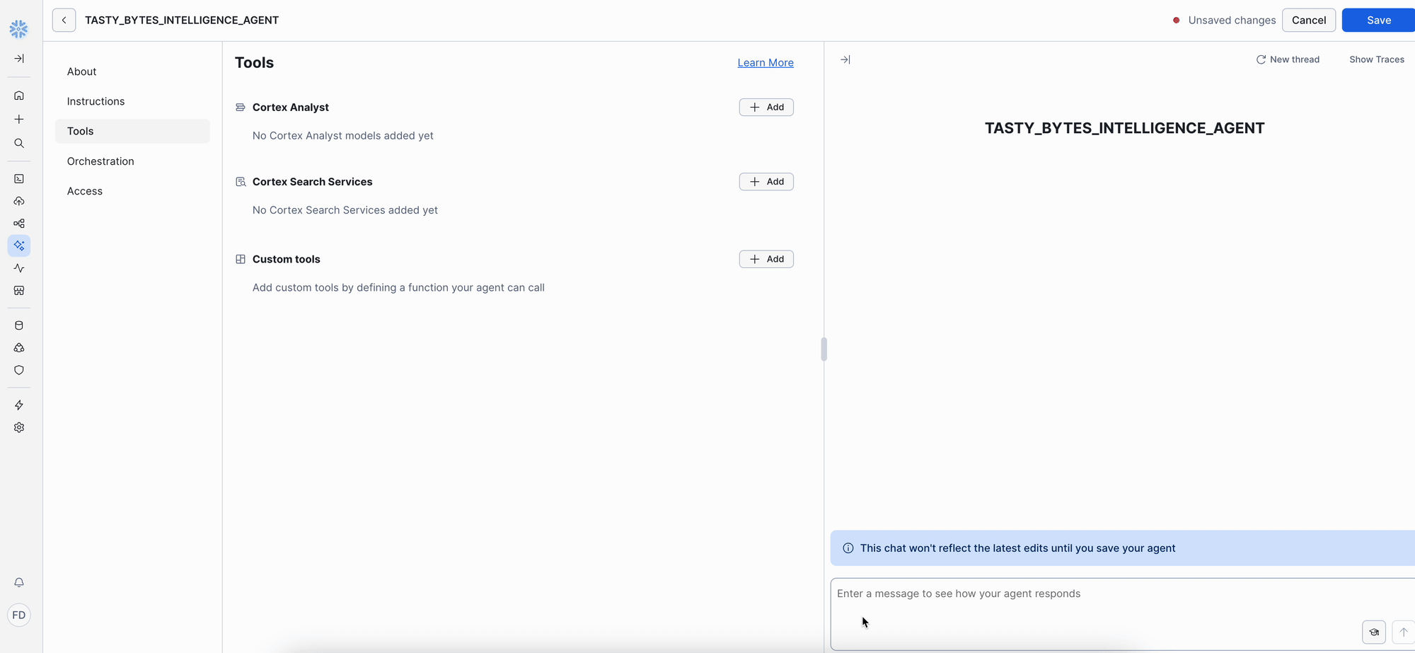
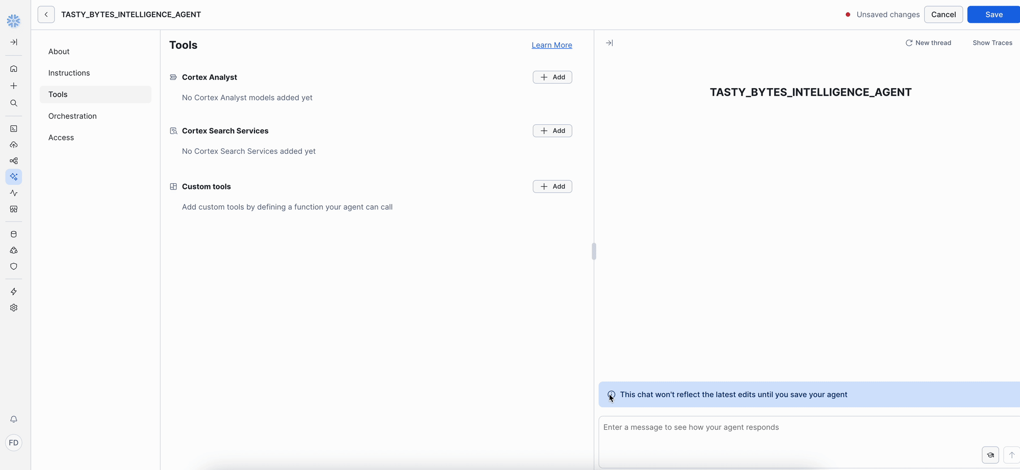
Add the Cortex Search Services Tool:
1. Click
Add
next to "Cortex Search Services."
2.
Configure tool details
:
Name
:
tasty_bytes_review_search
.
Description
:
Searches customer reviews and feedback to identify sentiment, operational issues, and customer satisfaction in
3.
Configure data source location
:
4.
Configure search result columns
:
5.
Configure search filters (optional)
:
6. Click
Add
.
Schema
: Choose
TB_101.HARMONIZED
.
Search service
: Choose
TB_101.HARMONIZED.TASTY_BYTES_REVIEW_SEARCH
.
ID column
: Select
Review
Title column
: Select
TRUCK_BRAND_NAME
Click
Add filter
to add up to 5 optional filters.
9/26/26, 12:02 PM
Zero to Snowflake
https://www.snowflake.com/en/developers/guides/zero-to-snowflake/
40/59
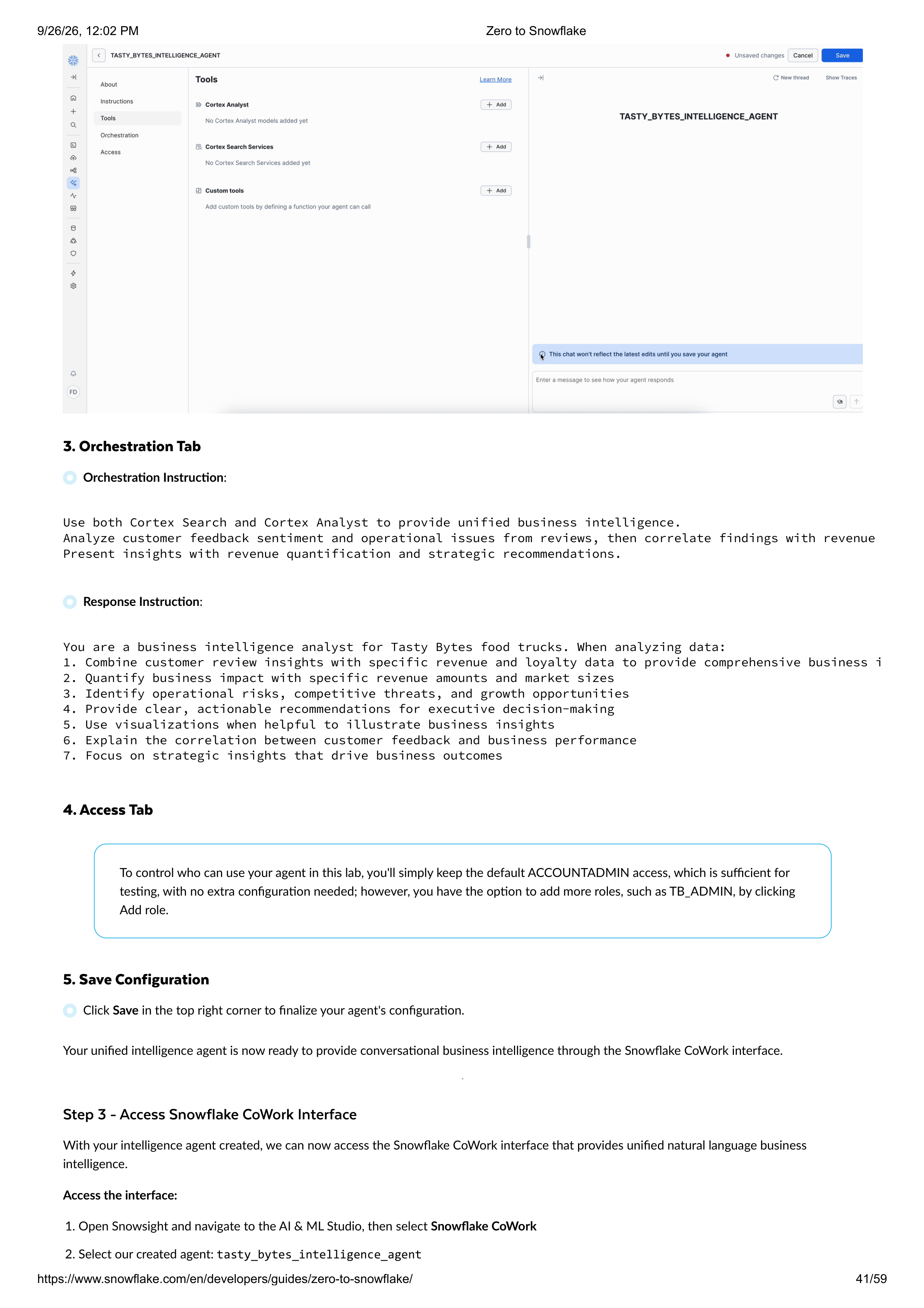
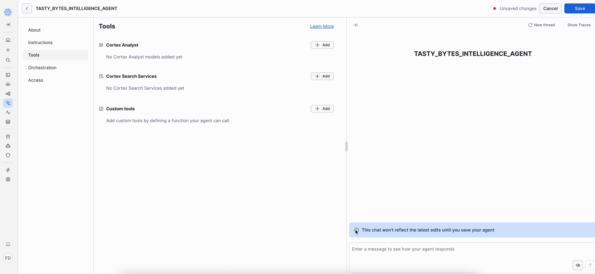
3. Orchestration Tab
4. Access Tab
5. Save Configuration
Step 3 - Access Snowflake CoWork Interface
Orchestration Instruction
:
Use both Cortex Search and Cortex Analyst to provide unified business intelligence.
Analyze customer feedback sentiment and operational issues from reviews, then correlate findings with revenue
Present insights with revenue quantification and strategic recommendations.
Response Instruction
:
You are a business intelligence analyst for Tasty Bytes food trucks. When analyzing data:
1. Combine customer review insights with specific revenue and loyalty data to provide comprehensive business i
2. Quantify business impact with specific revenue amounts and market sizes
3. Identify operational risks, competitive threats, and growth opportunities
4. Provide clear, actionable recommendations for executive decision-making
5. Use visualizations when helpful to illustrate business insights
6. Explain the correlation between customer feedback and business performance
7. Focus on strategic insights that drive business outcomes
To control who can use your agent in this lab, you'll simply keep the default ACCOUNTADMIN access, which is sufficient for
testing, with no extra configuration needed; however, you have the option to add more roles, such as TB_ADMIN, by clicking
Add role.
Click
Save
in the top right corner to finalize your agent's configuration.
Your unified intelligence agent is now ready to provide conversational business intelligence through the Snowflake CoWork interface.
With your intelligence agent created, we can now access the Snowflake CoWork interface that provides unified natural language business
intelligence.
Access the interface:
1. Open Snowsight and navigate to the AI & ML Studio, then select
Snowflake CoWork
2. Select our created agent:
tasty_bytes_intelligence_agent
9/26/26, 12:02 PM
Zero to Snowflake
https://www.snowflake.com/en/developers/guides/zero-to-snowflake/
41/59
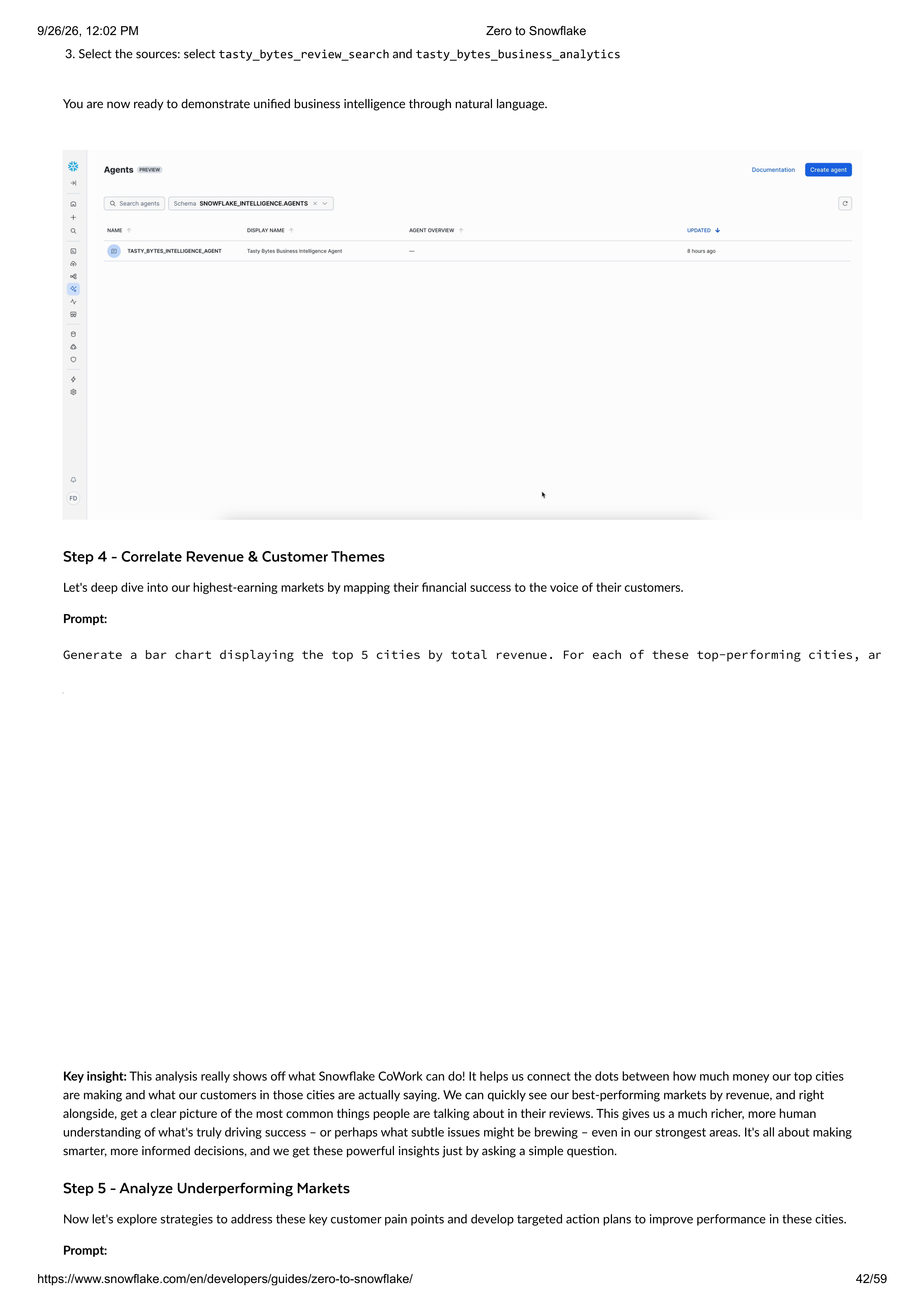
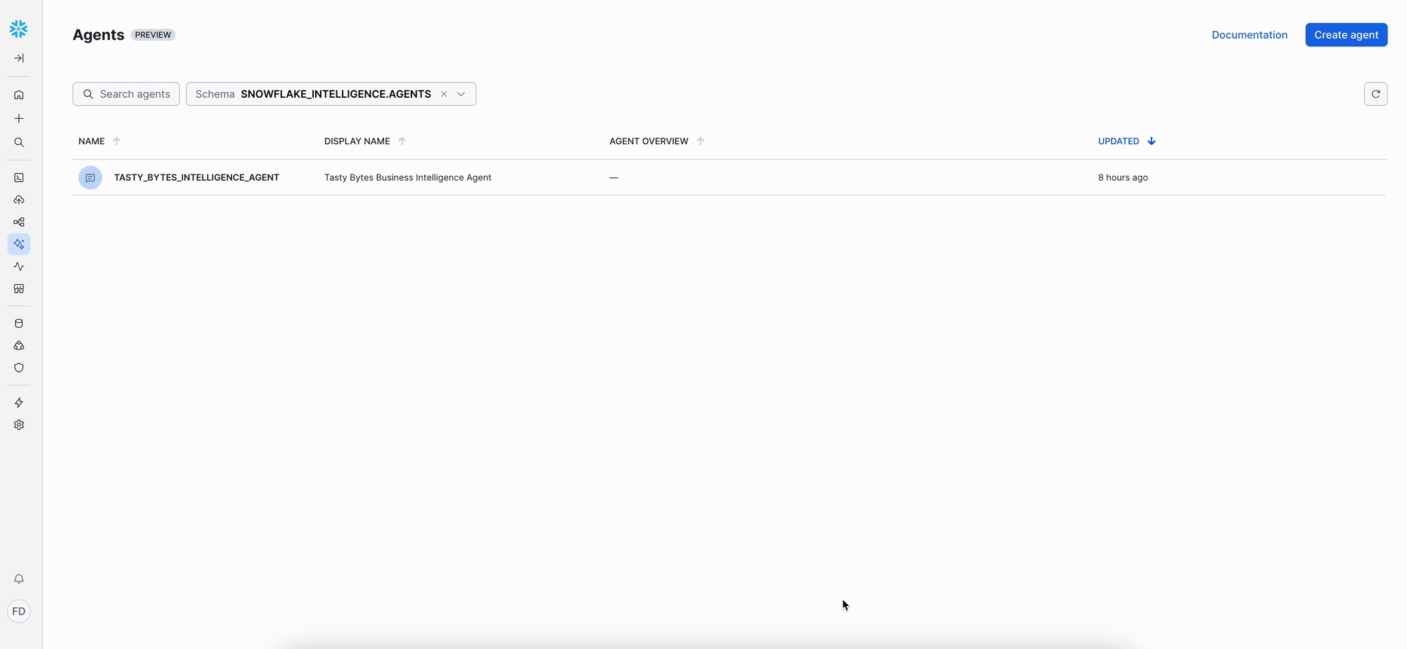

Step 4 - Correlate Revenue & Customer Themes
Step 5 - Analyze Underperforming Markets
3. Select the sources: select
tasty_bytes_review_search
and
tasty_bytes_business_analytics
You are now ready to demonstrate unified business intelligence through natural language.
Let's deep dive into our highest-earning markets by mapping their financial success to the voice of their customers.
Prompt:
Generate a bar chart displaying the top 5 cities by total revenue. For each of these top-performing cities, an
Key insight:
This analysis really shows off what Snowflake CoWork can do! It helps us connect the dots between how much money our top cities
are making and what our customers in those cities are actually saying. We can quickly see our best-performing markets by revenue, and right
alongside, get a clear picture of the most common things people are talking about in their reviews. This gives us a much richer, more human
understanding of what's truly driving success – or perhaps what subtle issues might be brewing – even in our strongest areas. It's all about making
smarter, more informed decisions, and we get these powerful insights just by asking a simple question.
Now let's explore strategies to address these key customer pain points and develop targeted action plans to improve performance in these cities.
Prompt:
9/26/26, 12:02 PM
Zero to Snowflake
https://www.snowflake.com/en/developers/guides/zero-to-snowflake/
42/59


Conclusion
Governance with Horizon
Overview
What You Will Learn
Identify the 5 cities with the lowest total revenue. For each of these cities, analyze their customer reviews
Key insight:
This analysis from Snowflake CoWork gives us a clear picture of our lowest-earning cities and, crucially, shines a light on the exact
customer pain points that are holding them back. By directly connecting raw revenue numbers with specific feedback from customer reviews, we
can pinpoint where we need to focus our efforts to improve service, product, or support. This provides actionable intelligence to drive targeted
growth and customer satisfaction in these challenged markets, all by simply asking a natural language question.
What we've just experienced with Tasty Bytes showcases a fundamental shift in how businesses can truly understand their data. By seamlessly
integrating Snowflake Cortex Search for deep dives into unstructured customer feedback and Cortex Analyst for conversational insights from
structured business metrics, we've brought a truly unified business intelligence to life.
You saw firsthand the power of this integration: users of all technical levels can now simply ask natural language questions and immediately receive
visually rich, actionable answers. This direct and intuitive access to insights fundamentally transforms how organizations can swiftly identify
operational risks, precisely quantify financial impact, and pinpoint new growth opportunities. It's clear that Snowflake CoWork empowers rapid,
data-driven decision-making, converting what was once fragmented data into clear, compelling business advantage for everyone.
Within this vignette, we will explore some of the powerful governance features within Snowflake Horizon. We will begin with a look at Role-Based
Access Control (RBAC), before diving into features like automated data classification, tag-based masking policies for column-level security, row-
access policies, data quality monitoring, and finally, account-wide security monitoring with the Trust Center.
The fundamentals of Role-Based Access Control (RBAC) in Snowflake.
9/26/26, 12:02 PM
Zero to Snowflake
https://www.snowflake.com/en/developers/guides/zero-to-snowflake/
43/59
What You Will Build
Get the SQL code and paste it into your SQL File.
Roles and Access Control
Overview
Step 1 - Set Context and View Existing Roles
Step 2 - Create a Custom Role
How to automatically classify and tag sensitive data.
How to implement column-level security with Dynamic Data Masking.
How to implement row-level security with Row Access Policies.
How to monitor data quality with Data Metric Functions.
How to monitor account security with the Trust Center.
A custom, privileged role.
A data classification profile for auto-tagging PII.
Tag-based masking policies for string and date columns.
A row access policy to restrict data visibility by country.
A custom Data Metric Function to check data integrity.
Copy and paste the SQL from this
file
in a new SQL File to follow along in Snowflake.
Note that once you've reached the end of the SQL File you can skip to
Step 29 - Apps & Collaboration
.
Snowflake's security model is built on a framework of Role-based Access Control (RBAC) and Discretionary Access Control (DAC). Access privileges
are assigned to roles, which are then assigned to users. This creates a powerful and flexible hierarchy for securing objects.
Access Control Overview
: To learn more about the key concepts of access control in Snowflake, including securable objects,
roles, privileges, and users.
First, let's set our context for this exercise and view the roles that already exist in the account.
USE ROLE useradmin;
USE ROLE useradmin;
USE DATABASE tb_101;
USE DATABASE tb_101;
USE WAREHOUSE tb_dev_wh;
USE WAREHOUSE tb_dev_wh;
SHOW ROLES;
SHOW ROLES;
We will now create a custom
tb_data_steward
role. This role will be responsible for managing and protecting our customer data.
CREATE OR REPLACE ROLE tb_data_steward
CREATE OR REPLACE ROLE tb_data_steward
COMMENT = 'Custom Role';
COMMENT = 'Custom Role';
The typical hierarchy of system and custom roles might look something like this:
+---------------+
| ACCOUNTADMIN |
+---------------+
^ ^ ^
| | |
+-------------+-+ | ++-------------+
| SECURITYADMIN | | | SYSADMIN |<------------+
+---------------+ | +--------------+ |
^ | ^ ^ |
9/26/26, 12:02 PM
Zero to Snowflake
https://www.snowflake.com/en/developers/guides/zero-to-snowflake/
44/59
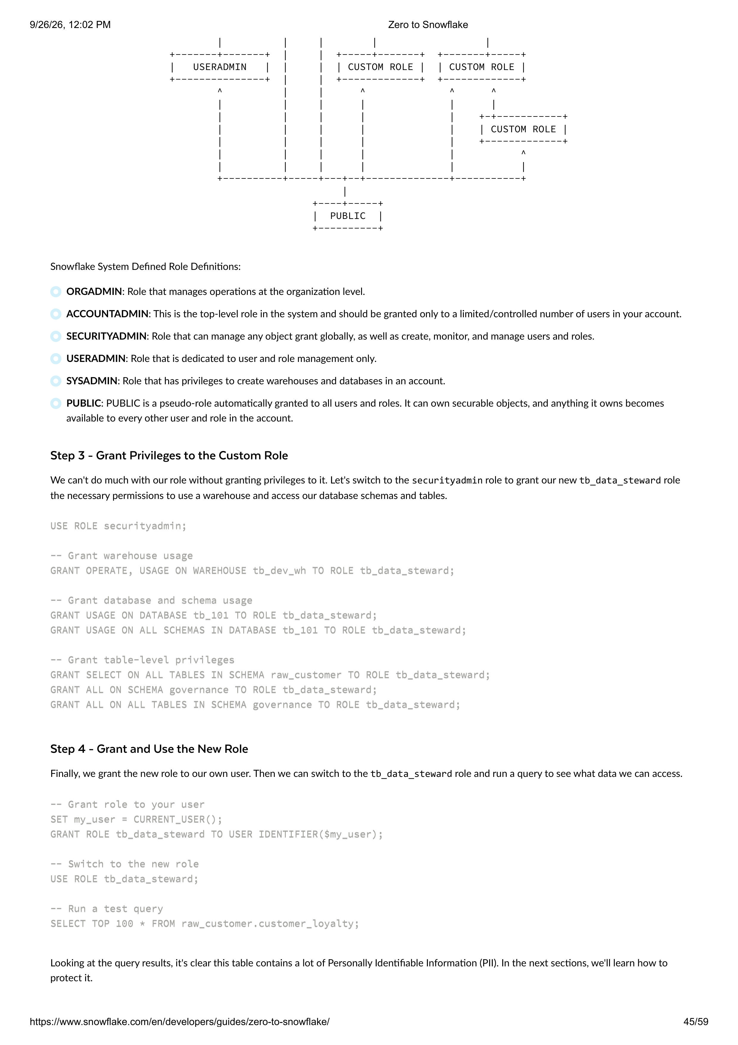
Step 3 - Grant Privileges to the Custom Role
Step 4 - Grant and Use the New Role
| | | | |
+-------+-------+ | | +-----+-------+ +-------+-----+
| USERADMIN | | | | CUSTOM ROLE | | CUSTOM ROLE |
+---------------+ | | +-------------+ +-------------+
^ | | ^ ^ ^
| | | | | |
| | | | | +-+-----------+
| | | | | | CUSTOM ROLE |
| | | | | +-------------+
| | | | | ^
| | | | | |
+----------+-----+---+--+--------------+-----------+
|
+----+-----+
| PUBLIC |
+----------+
Snowflake System Defined Role Definitions:
ORGADMIN
: Role that manages operations at the organization level.
ACCOUNTADMIN
: This is the top-level role in the system and should be granted only to a limited/controlled number of users in your account.
SECURITYADMIN
: Role that can manage any object grant globally, as well as create, monitor, and manage users and roles.
USERADMIN
: Role that is dedicated to user and role management only.
SYSADMIN
: Role that has privileges to create warehouses and databases in an account.
PUBLIC
: PUBLIC is a pseudo-role automatically granted to all users and roles. It can own securable objects, and anything it owns becomes
available to every other user and role in the account.
We can't do much with our role without granting privileges to it. Let's switch to the
securityadmin
role to grant our new
tb_data_steward
role
the necessary permissions to use a warehouse and access our database schemas and tables.
USE ROLE securityadmin;
USE ROLE securityadmin;
-- Grant warehouse usage
-- Grant warehouse usage
GRANT OPERATE, USAGE ON WAREHOUSE tb_dev_wh TO ROLE tb_data_steward;
GRANT OPERATE, USAGE ON WAREHOUSE tb_dev_wh TO ROLE tb_data_steward;
-- Grant database and schema usage
-- Grant database and schema usage
GRANT USAGE ON DATABASE tb_101 TO ROLE tb_data_steward;
GRANT USAGE ON DATABASE tb_101 TO ROLE tb_data_steward;
GRANT USAGE ON ALL SCHEMAS IN DATABASE tb_101 TO ROLE tb_data_steward;
GRANT USAGE ON ALL SCHEMAS IN DATABASE tb_101 TO ROLE tb_data_steward;
-- Grant table-level privileges
-- Grant table-level privileges
GRANT SELECT ON ALL TABLES IN SCHEMA raw_customer TO ROLE tb_data_steward;
GRANT SELECT ON ALL TABLES IN SCHEMA raw_customer TO ROLE tb_data_steward;
GRANT ALL ON SCHEMA governance TO ROLE tb_data_steward;
GRANT ALL ON SCHEMA governance TO ROLE tb_data_steward;
GRANT ALL ON ALL TABLES IN SCHEMA governance TO ROLE tb_data_steward;
GRANT ALL ON ALL TABLES IN SCHEMA governance TO ROLE tb_data_steward;
Finally, we grant the new role to our own user. Then we can switch to the
tb_data_steward
role and run a query to see what data we can access.
-- Grant role to your user
-- Grant role to your user
SET my_user = CURRENT_USER();
SET my_user = CURRENT_USER();
GRANT ROLE tb_data_steward TO USER IDENTIFIER($my_user);
GRANT ROLE tb_data_steward TO USER IDENTIFIER($my_user);
-- Switch to the new role
-- Switch to the new role
USE ROLE tb_data_steward;
USE ROLE tb_data_steward;
-- Run a test query
-- Run a test query
SELECT TOP 100 * FROM raw_customer.customer_loyalty;
SELECT TOP 100 * FROM raw_customer.customer_loyalty;
Looking at the query results, it's clear this table contains a lot of Personally Identifiable Information (PII). In the next sections, we'll learn how to
protect it.
9/26/26, 12:02 PM
Zero to Snowflake
https://www.snowflake.com/en/developers/guides/zero-to-snowflake/
45/59
Classification and Auto Tagging
Overview
Step 1 - Create PII Tag and Grant Privileges
Step 2 - Create a Classification Profile
Step 3 - Map Semantic Categories to the PII Tag
Step 4 - Run Classification and View Results
A key first step in data governance is identifying and classifying sensitive data. Snowflake Horizon's auto-tagging capability can automatically
discover sensitive information by monitoring columns in your schemas. We can then use these tags to apply security policies.
Automatic Classification
: Learn how Snowflake can automatically classify sensitive data based on a schedule, simplifying
governance at scale.
Using the
accountadmin
role, we'll create a
pii
tag in our
governance
schema. We will also grant the necessary privileges to our
tb_data_steward
role to perform classification.
USE ROLE accountadmin;
USE ROLE accountadmin;
CREATE OR REPLACE TAG governance.pii;
CREATE OR REPLACE TAG governance.pii;
GRANT APPLY TAG ON ACCOUNT TO ROLE tb_data_steward;
GRANT APPLY TAG ON ACCOUNT TO ROLE tb_data_steward;
GRANT EXECUTE AUTO CLASSIFICATION ON SCHEMA raw_customer TO ROLE tb_data_steward;
GRANT EXECUTE AUTO CLASSIFICATION ON SCHEMA raw_customer TO ROLE tb_data_steward;
GRANT DATABASE ROLE SNOWFLAKE.CLASSIFICATION_ADMIN TO ROLE tb_data_steward;
GRANT DATABASE ROLE SNOWFLAKE.CLASSIFICATION_ADMIN TO ROLE tb_data_steward;
GRANT CREATE SNOWFLAKE.DATA_PRIVACY.CLASSIFICATION_PROFILE ON SCHEMA governance TO ROLE tb_data_steward;
GRANT CREATE SNOWFLAKE.DATA_PRIVACY.CLASSIFICATION_PROFILE ON SCHEMA governance TO ROLE tb_data_steward;
Now, as the
tb_data_steward
, we'll create a classification profile. This profile defines how auto-tagging will behave.
USE ROLE tb_data_steward;
USE ROLE tb_data_steward;
CREATE OR REPLACE SNOWFLAKE.DATA_PRIVACY.CLASSIFICATION_PROFILE
CREATE OR REPLACE SNOWFLAKE.DATA_PRIVACY.CLASSIFICATION_PROFILE
governance.tb_classification_profile(
governance.tb_classification_profile(
{
{
'minimum_object_age_for_classification_days': 0,
'minimum_object_age_for_classification_days': 0,
'maximum_classification_validity_days': 30,
'maximum_classification_validity_days': 30,
'auto_tag': true
'auto_tag': true
});
});
Next, we'll define a mapping that tells the classification profile to apply our
governance.pii
tag to any column whose
SEMANTIC_CATEGORY
matches common PII types like
NAME
,
PHONE_NUMBER
,
EMAIL
, etc.
CALL governance.tb_classification_profile!SET_TAG_MAP(
CALL governance.tb_classification_profile!SET_TAG_MAP(
{'column_tag_map':[
{'column_tag_map':[
{
{
'tag_name':'tb_101.governance.pii',
'tag_name':'tb_101.governance.pii',
'tag_value':'pii',
'tag_value':'pii',
'semantic_categories':['NAME', 'PHONE_NUMBER', 'POSTAL_CODE', 'DATE_OF_BIRTH', 'CITY', 'EMAIL']
'semantic_categories':['NAME', 'PHONE_NUMBER', 'POSTAL_CODE', 'DATE_OF_BIRTH', 'CITY', 'EMAIL']
}]});
}]});
Let's manually trigger the classification process on our
customer_loyalty
table. Then, we can query the
INFORMATION_SCHEMA
to see the tags
that were automatically applied.
-- Trigger classification
-- Trigger classification
CALL SYSTEM$CLASSIFY('tb_101.raw_customer.customer_loyalty', 'tb_101.governance.tb_classification_profile');
CALL SYSTEM$CLASSIFY('tb_101.raw_customer.customer_loyalty', 'tb_101.governance.tb_classification_profile');
-- View applied tags
-- View applied tags
9/26/26, 12:02 PM
Zero to Snowflake
https://www.snowflake.com/en/developers/guides/zero-to-snowflake/
46/59
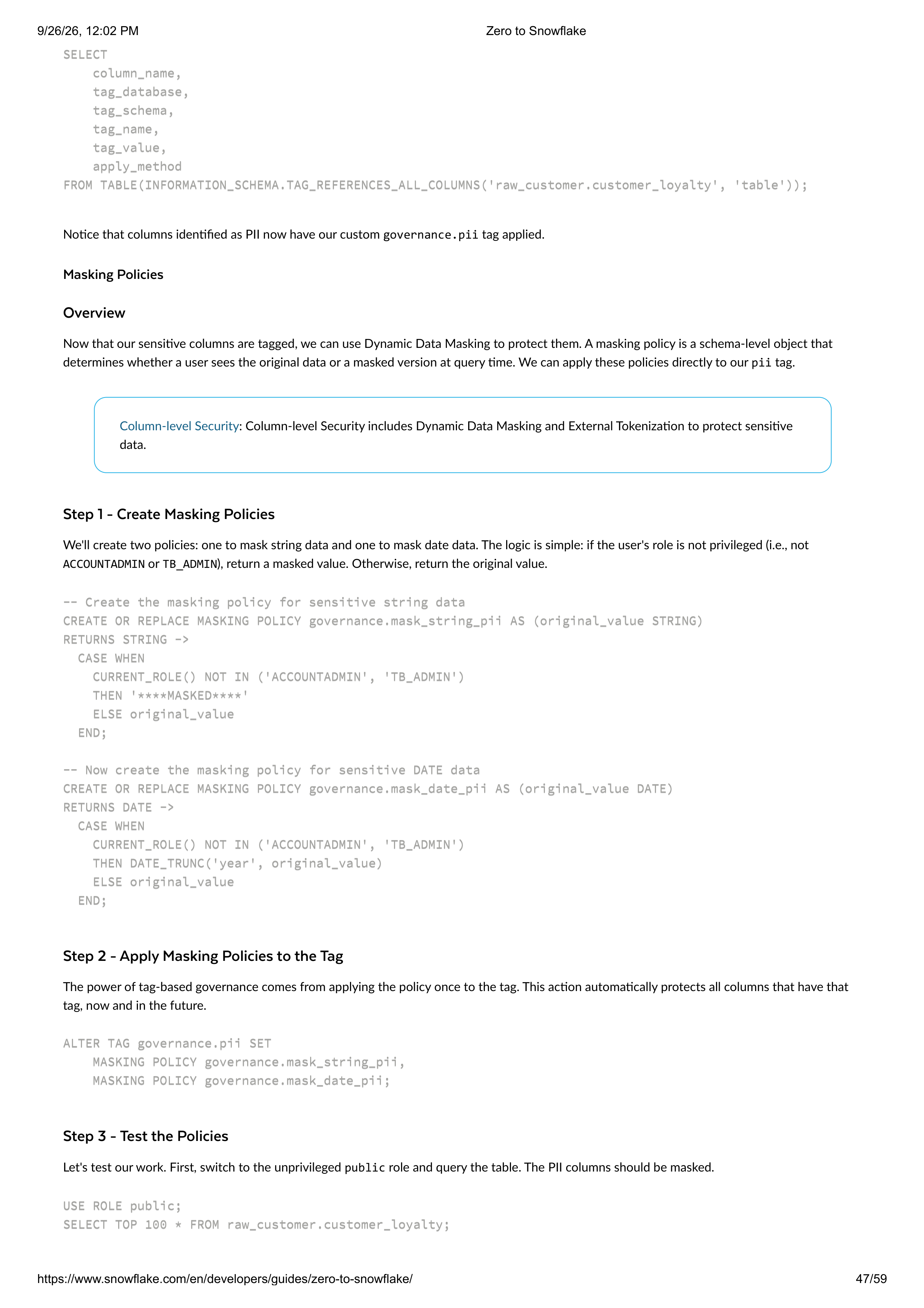
Masking Policies
Overview
Step 1 - Create Masking Policies
Step 2 - Apply Masking Policies to the Tag
Step 3 - Test the Policies
SELECT
SELECT
column_name,
column_name,
tag_database,
tag_database,
tag_schema,
tag_schema,
tag_name,
tag_name,
tag_value,
tag_value,
apply_method
apply_method
FROM TABLE(INFORMATION_SCHEMA.TAG_REFERENCES_ALL_COLUMNS('raw_customer.customer_loyalty', 'table'));
FROM TABLE(INFORMATION_SCHEMA.TAG_REFERENCES_ALL_COLUMNS('raw_customer.customer_loyalty', 'table'));
Notice that columns identified as PII now have our custom
governance.pii
tag applied.
Now that our sensitive columns are tagged, we can use Dynamic Data Masking to protect them. A masking policy is a schema-level object that
determines whether a user sees the original data or a masked version at query time. We can apply these policies directly to our
pii
tag.
Column-level Security
: Column-level Security includes Dynamic Data Masking and External Tokenization to protect sensitive
data.
We'll create two policies: one to mask string data and one to mask date data. The logic is simple: if the user's role is not privileged (i.e., not
ACCOUNTADMIN
or
TB_ADMIN
), return a masked value. Otherwise, return the original value.
-- Create the masking policy for sensitive string data
-- Create the masking policy for sensitive string data
CREATE OR REPLACE MASKING POLICY governance.mask_string_pii AS (original_value STRING)
CREATE OR REPLACE MASKING POLICY governance.mask_string_pii AS (original_value STRING)
RETURNS STRING ->
RETURNS STRING ->
CASE WHEN
CASE WHEN
CURRENT_ROLE() NOT IN ('ACCOUNTADMIN', 'TB_ADMIN')
CURRENT_ROLE() NOT IN ('ACCOUNTADMIN', 'TB_ADMIN')
THEN '****MASKED****'
THEN '****MASKED****'
ELSE original_value
ELSE original_value
END;
END;
-- Now create the masking policy for sensitive DATE data
-- Now create the masking policy for sensitive DATE data
CREATE OR REPLACE MASKING POLICY governance.mask_date_pii AS (original_value DATE)
CREATE OR REPLACE MASKING POLICY governance.mask_date_pii AS (original_value DATE)
RETURNS DATE ->
RETURNS DATE ->
CASE WHEN
CASE WHEN
CURRENT_ROLE() NOT IN ('ACCOUNTADMIN', 'TB_ADMIN')
CURRENT_ROLE() NOT IN ('ACCOUNTADMIN', 'TB_ADMIN')
THEN DATE_TRUNC('year', original_value)
THEN DATE_TRUNC('year', original_value)
ELSE original_value
ELSE original_value
END;
END;
The power of tag-based governance comes from applying the policy once to the tag. This action automatically protects all columns that have that
tag, now and in the future.
ALTER TAG governance.pii SET
ALTER TAG governance.pii SET
MASKING POLICY governance.mask_string_pii,
MASKING POLICY governance.mask_string_pii,
MASKING POLICY governance.mask_date_pii;
MASKING POLICY governance.mask_date_pii;
Let's test our work. First, switch to the unprivileged
public
role and query the table. The PII columns should be masked.
USE ROLE public;
USE ROLE public;
SELECT TOP 100 * FROM raw_customer.customer_loyalty;
SELECT TOP 100 * FROM raw_customer.customer_loyalty;
9/26/26, 12:02 PM
Zero to Snowflake
https://www.snowflake.com/en/developers/guides/zero-to-snowflake/
47/59
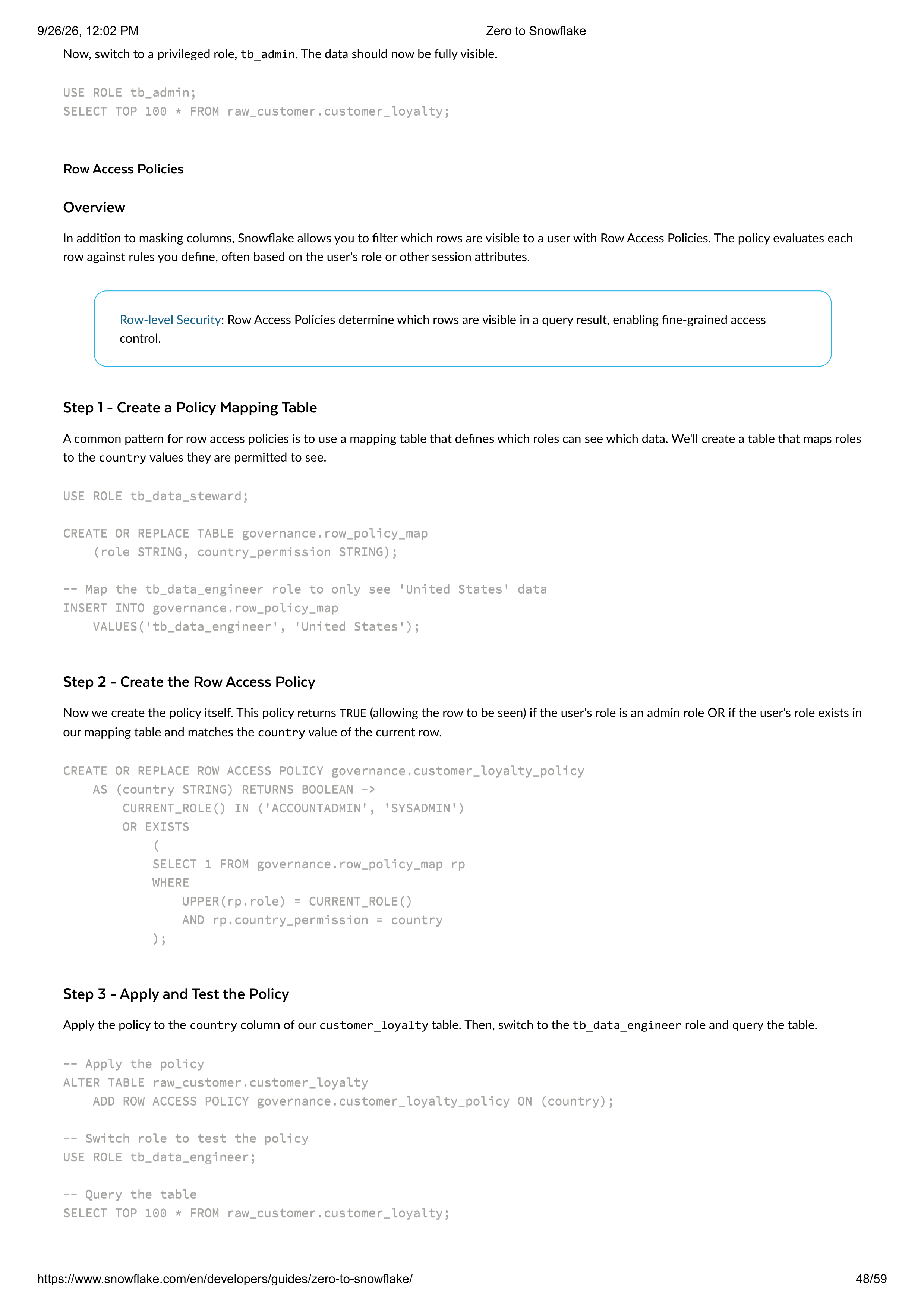
Row Access Policies
Overview
Step 1 - Create a Policy Mapping Table
Step 2 - Create the Row Access Policy
Step 3 - Apply and Test the Policy
Now, switch to a privileged role,
tb_admin
. The data should now be fully visible.
USE ROLE tb_admin;
USE ROLE tb_admin;
SELECT TOP 100 * FROM raw_customer.customer_loyalty;
SELECT TOP 100 * FROM raw_customer.customer_loyalty;
In addition to masking columns, Snowflake allows you to filter which rows are visible to a user with Row Access Policies. The policy evaluates each
row against rules you define, often based on the user's role or other session attributes.
Row-level Security
: Row Access Policies determine which rows are visible in a query result, enabling fine-grained access
control.
A common pattern for row access policies is to use a mapping table that defines which roles can see which data. We'll create a table that maps roles
to the
country
values they are permitted to see.
USE ROLE tb_data_steward;
USE ROLE tb_data_steward;
CREATE OR REPLACE TABLE governance.row_policy_map
CREATE OR REPLACE TABLE governance.row_policy_map
(role STRING, country_permission STRING);
(role STRING, country_permission STRING);
-- Map the tb_data_engineer role to only see 'United States' data
-- Map the tb_data_engineer role to only see 'United States' data
INSERT INTO governance.row_policy_map
INSERT INTO governance.row_policy_map
VALUES('tb_data_engineer', 'United States');
VALUES('tb_data_engineer', 'United States');
Now we create the policy itself. This policy returns
TRUE
(allowing the row to be seen) if the user's role is an admin role OR if the user's role exists in
our mapping table and matches the
country
value of the current row.
CREATE OR REPLACE ROW ACCESS POLICY governance.customer_loyalty_policy
CREATE OR REPLACE ROW ACCESS POLICY governance.customer_loyalty_policy
AS (country STRING) RETURNS BOOLEAN ->
AS (country STRING) RETURNS BOOLEAN ->
CURRENT_ROLE() IN ('ACCOUNTADMIN', 'SYSADMIN')
CURRENT_ROLE() IN ('ACCOUNTADMIN', 'SYSADMIN')
OR EXISTS
OR EXISTS
(
(
SELECT 1 FROM governance.row_policy_map rp
SELECT 1 FROM governance.row_policy_map rp
WHERE
WHERE
UPPER(rp.role) = CURRENT_ROLE()
UPPER(rp.role) = CURRENT_ROLE()
AND rp.country_permission = country
AND rp.country_permission = country
);
);
Apply the policy to the
country
column of our
customer_loyalty
table. Then, switch to the
tb_data_engineer
role and query the table.
-- Apply the policy
-- Apply the policy
ALTER TABLE raw_customer.customer_loyalty
ALTER TABLE raw_customer.customer_loyalty
ADD ROW ACCESS POLICY governance.customer_loyalty_policy ON (country);
ADD ROW ACCESS POLICY governance.customer_loyalty_policy ON (country);
-- Switch role to test the policy
-- Switch role to test the policy
USE ROLE tb_data_engineer;
USE ROLE tb_data_engineer;
-- Query the table
-- Query the table
SELECT TOP 100 * FROM raw_customer.customer_loyalty;
SELECT TOP 100 * FROM raw_customer.customer_loyalty;
9/26/26, 12:02 PM
Zero to Snowflake
https://www.snowflake.com/en/developers/guides/zero-to-snowflake/
48/59
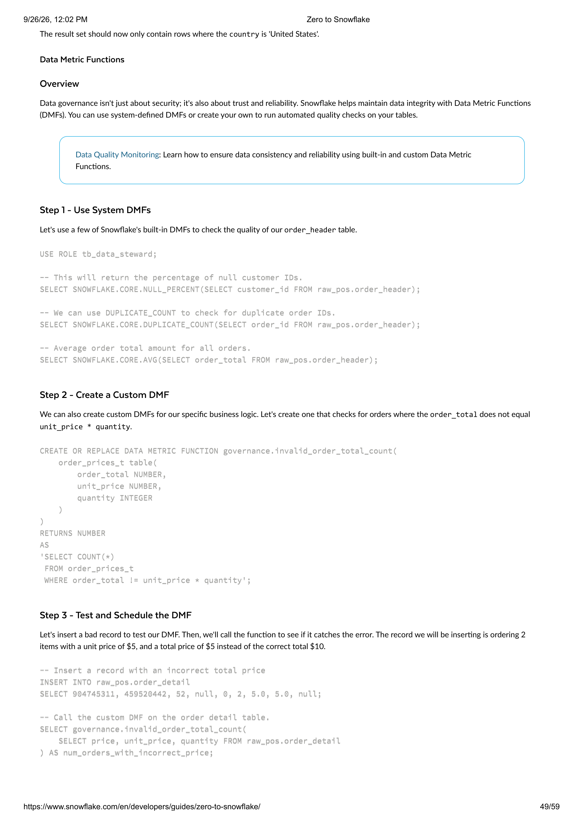
Data Metric Functions
Overview
Step 1 - Use System DMFs
Step 2 - Create a Custom DMF
Step 3 - Test and Schedule the DMF
The result set should now only contain rows where the
country
is 'United States'.
Data governance isn't just about security; it's also about trust and reliability. Snowflake helps maintain data integrity with Data Metric Functions
(DMFs). You can use system-defined DMFs or create your own to run automated quality checks on your tables.
Data Quality Monitoring
: Learn how to ensure data consistency and reliability using built-in and custom Data Metric
Functions.
Let's use a few of Snowflake's built-in DMFs to check the quality of our
order_header
table.
USE ROLE tb_data_steward;
USE ROLE tb_data_steward;
-- This will return the percentage of null customer IDs.
-- This will return the percentage of null customer IDs.
SELECT SNOWFLAKE.CORE.NULL_PERCENT(SELECT customer_id FROM raw_pos.order_header);
SELECT SNOWFLAKE.CORE.NULL_PERCENT(SELECT customer_id FROM raw_pos.order_header);
-- We can use DUPLICATE_COUNT to check for duplicate order IDs.
-- We can use DUPLICATE_COUNT to check for duplicate order IDs.
SELECT SNOWFLAKE.CORE.DUPLICATE_COUNT(SELECT order_id FROM raw_pos.order_header);
SELECT SNOWFLAKE.CORE.DUPLICATE_COUNT(SELECT order_id FROM raw_pos.order_header);
-- Average order total amount for all orders.
-- Average order total amount for all orders.
SELECT SNOWFLAKE.CORE.AVG(SELECT order_total FROM raw_pos.order_header);
SELECT SNOWFLAKE.CORE.AVG(SELECT order_total FROM raw_pos.order_header);
We can also create custom DMFs for our specific business logic. Let's create one that checks for orders where the
order_total
does not equal
unit_price * quantity
.
CREATE OR REPLACE DATA METRIC FUNCTION governance.invalid_order_total_count(
CREATE OR REPLACE DATA METRIC FUNCTION governance.invalid_order_total_count(
order_prices_t table(
order_prices_t table(
order_total NUMBER,
order_total NUMBER,
unit_price NUMBER,
unit_price NUMBER,
quantity INTEGER
quantity INTEGER
)
)
)
RETURNS NUMBER
RETURNS NUMBER
AS
AS
'SELECT COUNT(*)
'SELECT COUNT(*)
FROM order_prices_t
FROM order_prices_t
WHERE order_total != unit_price * quantity';
WHERE order_total != unit_price * quantity';
Let's insert a bad record to test our DMF. Then, we'll call the function to see if it catches the error. The record we will be inserting is ordering 2
items with a unit price of $5, and a total price of $5 instead of the correct total $10.
-- Insert a record with an incorrect total price
-- Insert a record with an incorrect total price
INSERT INTO raw_pos.order_detail
INSERT INTO raw_pos.order_detail
SELECT 904745311, 459520442, 52, null, 0, 2, 5.0, 5.0, null;
SELECT 904745311, 459520442, 52, null, 0, 2, 5.0, 5.0, null;
-- Call the custom DMF on the order detail table.
-- Call the custom DMF on the order detail table.
SELECT governance.invalid_order_total_count(
SELECT governance.invalid_order_total_count(
SELECT price, unit_price, quantity FROM raw_pos.order_detail
SELECT price, unit_price, quantity FROM raw_pos.order_detail
) AS num_orders_with_incorrect_price;
) AS num_orders_with_incorrect_price;
9/26/26, 12:02 PM
Zero to Snowflake
https://www.snowflake.com/en/developers/guides/zero-to-snowflake/
49/59
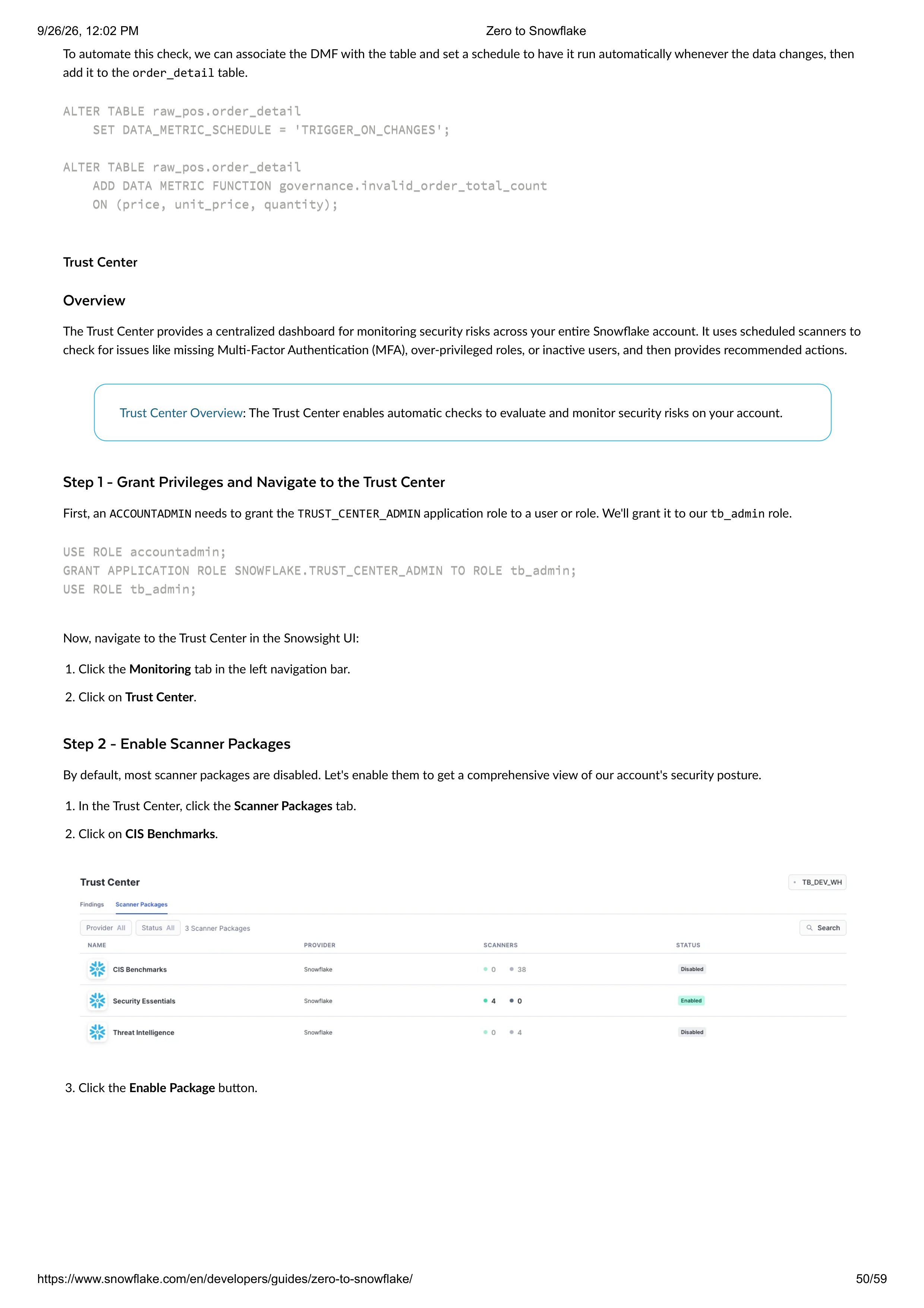
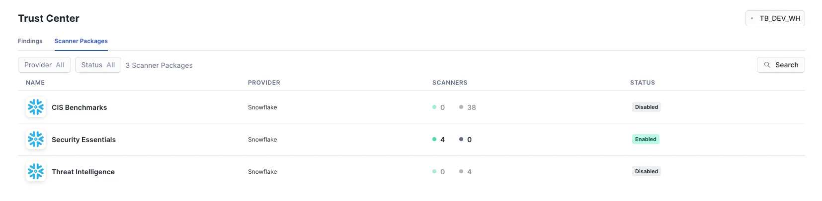
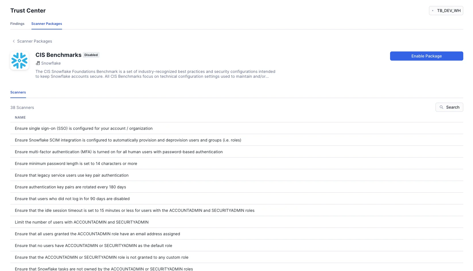
Trust Center
Overview
Step 1 - Grant Privileges and Navigate to the Trust Center
Step 2 - Enable Scanner Packages
To automate this check, we can associate the DMF with the table and set a schedule to have it run automatically whenever the data changes, then
add it to the
order_detail
table.
ALTER TABLE raw_pos.order_detail
ALTER TABLE raw_pos.order_detail
SET DATA_METRIC_SCHEDULE = 'TRIGGER_ON_CHANGES';
SET DATA_METRIC_SCHEDULE = 'TRIGGER_ON_CHANGES';
ALTER TABLE raw_pos.order_detail
ALTER TABLE raw_pos.order_detail
ADD DATA METRIC FUNCTION governance.invalid_order_total_count
ADD DATA METRIC FUNCTION governance.invalid_order_total_count
ON (price, unit_price, quantity);
ON (price, unit_price, quantity);
The Trust Center provides a centralized dashboard for monitoring security risks across your entire Snowflake account. It uses scheduled scanners to
check for issues like missing Multi-Factor Authentication (MFA), over-privileged roles, or inactive users, and then provides recommended actions.
Trust Center Overview
: The Trust Center enables automatic checks to evaluate and monitor security risks on your account.
First, an
ACCOUNTADMIN
needs to grant the
TRUST_CENTER_ADMIN
application role to a user or role. We'll grant it to our
tb_admin
role.
USE ROLE accountadmin;
USE ROLE accountadmin;
GRANT APPLICATION ROLE SNOWFLAKE.TRUST_CENTER_ADMIN TO ROLE tb_admin;
GRANT APPLICATION ROLE SNOWFLAKE.TRUST_CENTER_ADMIN TO ROLE tb_admin;
USE ROLE tb_admin;
USE ROLE tb_admin;
Now, navigate to the Trust Center in the Snowsight UI:
1. Click the
Monitoring
tab in the left navigation bar.
2. Click on
Trust Center
.
By default, most scanner packages are disabled. Let's enable them to get a comprehensive view of our account's security posture.
1. In the Trust Center, click the
Scanner Packages
tab.
2. Click on
CIS Benchmarks
.
3. Click the
Enable Package
button.
9/26/26, 12:02 PM
Zero to Snowflake
https://www.snowflake.com/en/developers/guides/zero-to-snowflake/
50/59
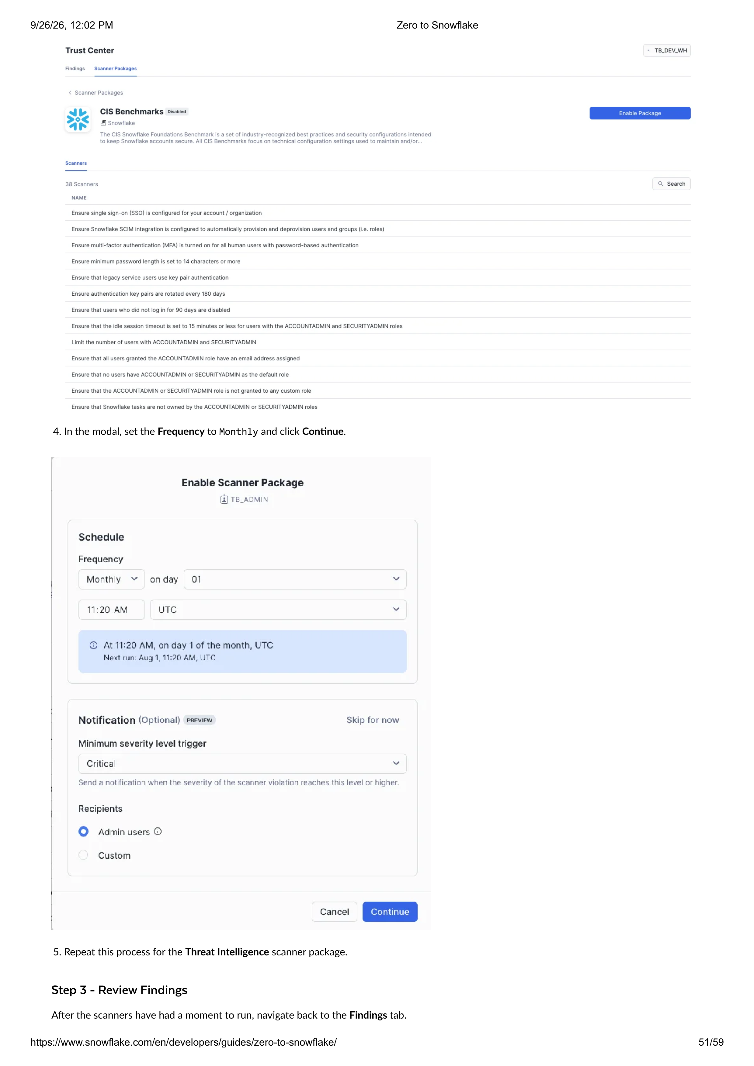
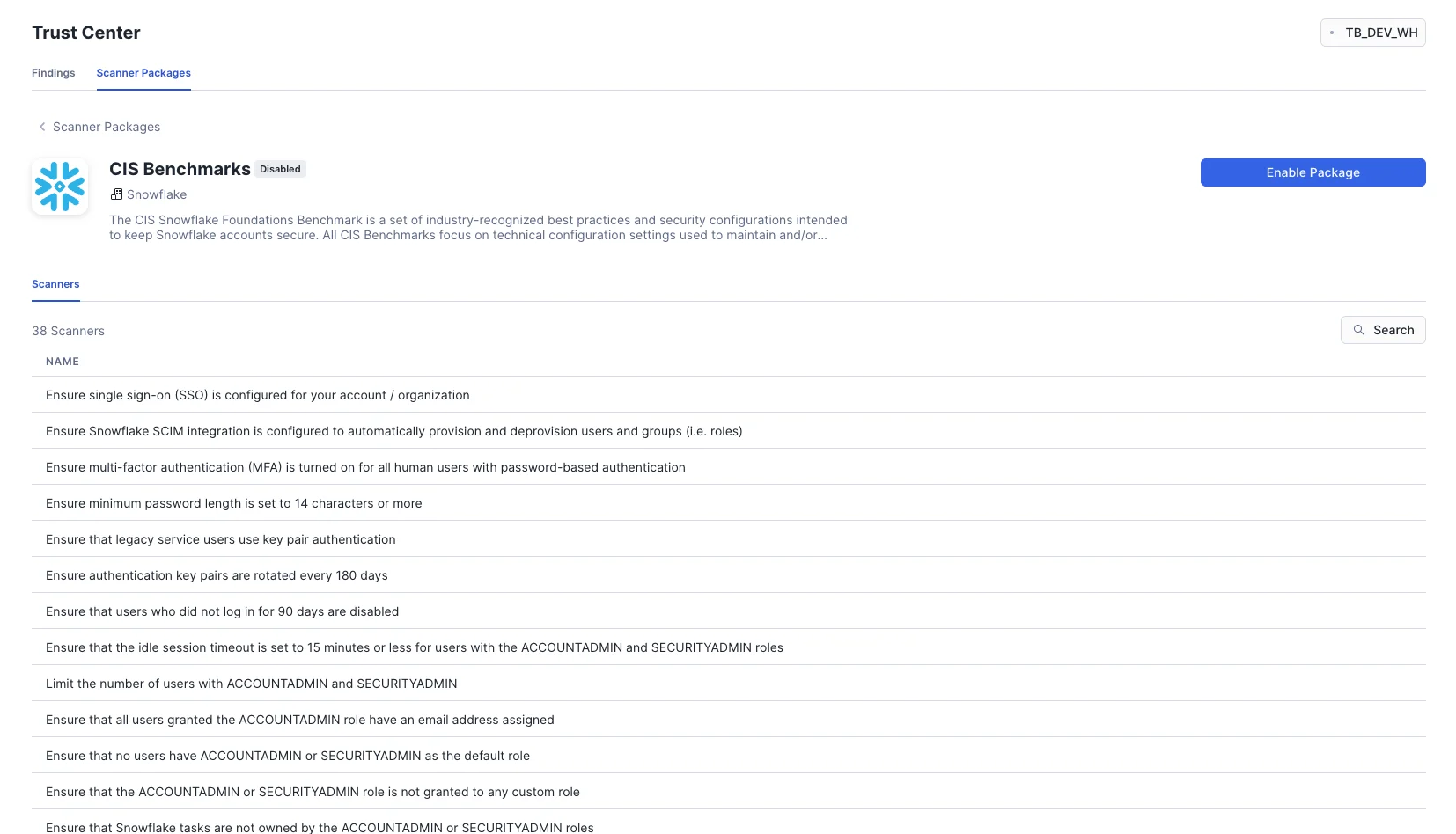
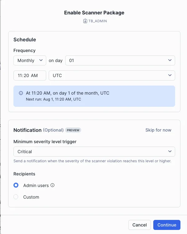
Step 3 - Review Findings
4. In the modal, set the
Frequency
to
Monthly
and click
Continue
.
5. Repeat this process for the
Threat Intelligence
scanner package.
After the scanners have had a moment to run, navigate back to the
Findings
tab.
9/26/26, 12:02 PM
Zero to Snowflake
https://www.snowflake.com/en/developers/guides/zero-to-snowflake/
51/59
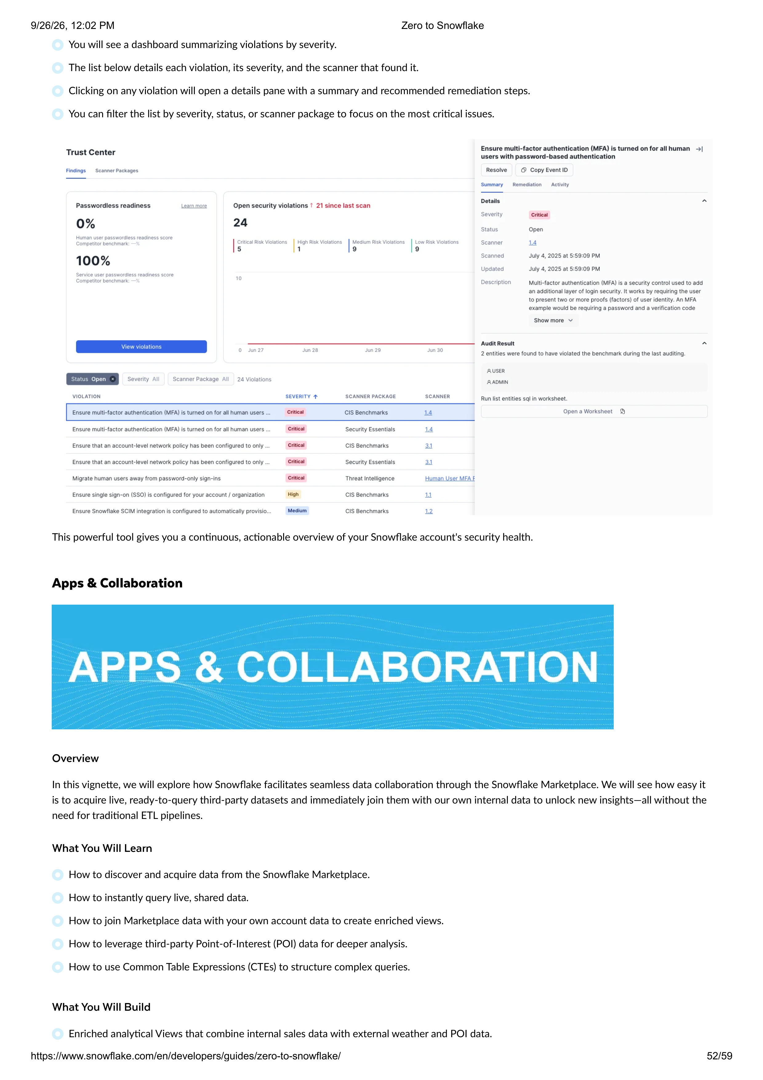
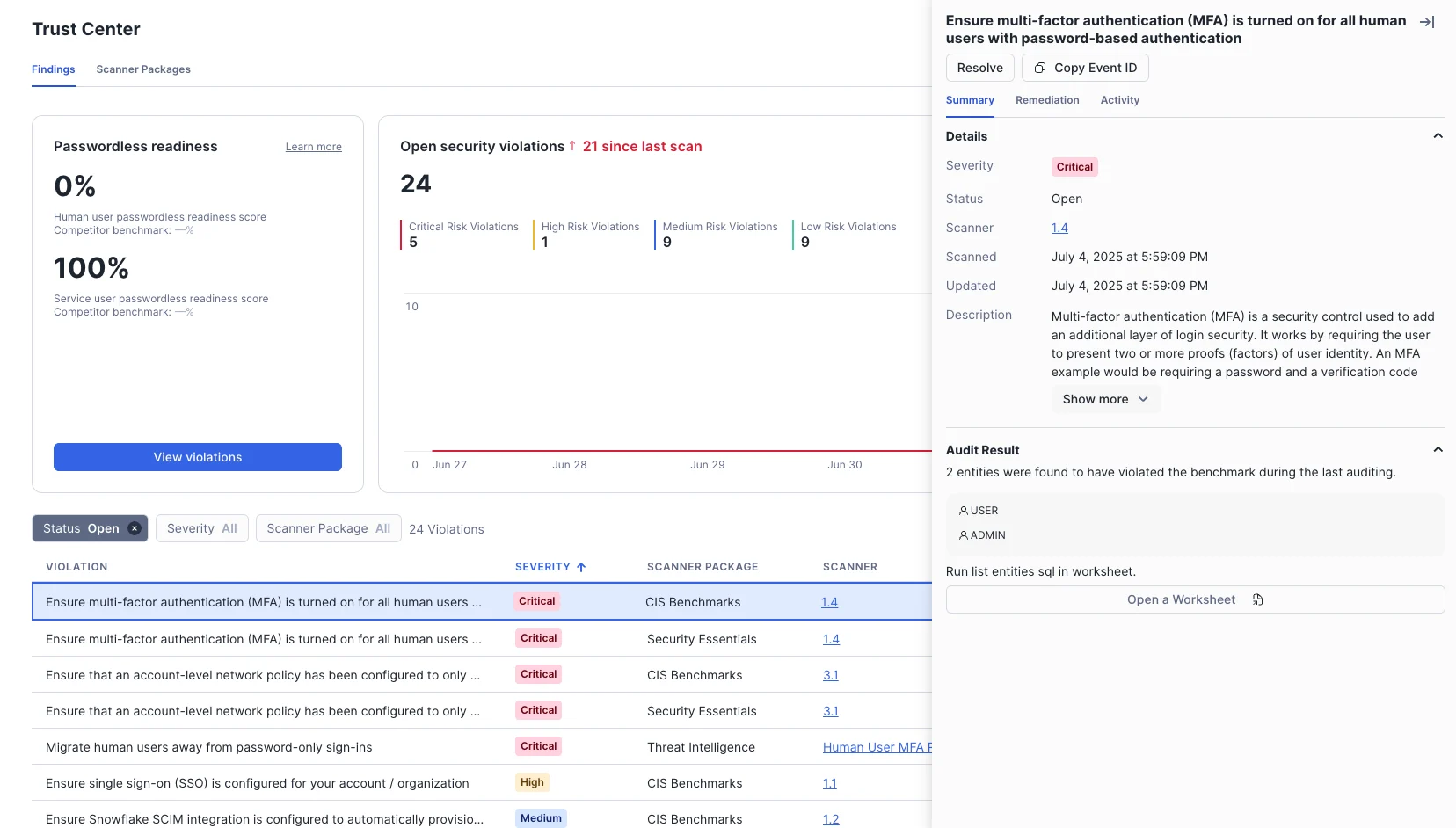

Apps & Collaboration
Overview
What You Will Learn
What You Will Build
You will see a dashboard summarizing violations by severity.
The list below details each violation, its severity, and the scanner that found it.
Clicking on any violation will open a details pane with a summary and recommended remediation steps.
You can filter the list by severity, status, or scanner package to focus on the most critical issues.
This powerful tool gives you a continuous, actionable overview of your Snowflake account's security health.
In this vignette, we will explore how Snowflake facilitates seamless data collaboration through the Snowflake Marketplace. We will see how easy it
is to acquire live, ready-to-query third-party datasets and immediately join them with our own internal data to unlock new insights—all without the
need for traditional ETL pipelines.
How to discover and acquire data from the Snowflake Marketplace.
How to instantly query live, shared data.
How to join Marketplace data with your own account data to create enriched views.
How to leverage third-party Point-of-Interest (POI) data for deeper analysis.
How to use Common Table Expressions (CTEs) to structure complex queries.
Enriched analytical Views that combine internal sales data with external weather and POI data.
9/26/26, 12:02 PM
Zero to Snowflake
https://www.snowflake.com/en/developers/guides/zero-to-snowflake/
52/59
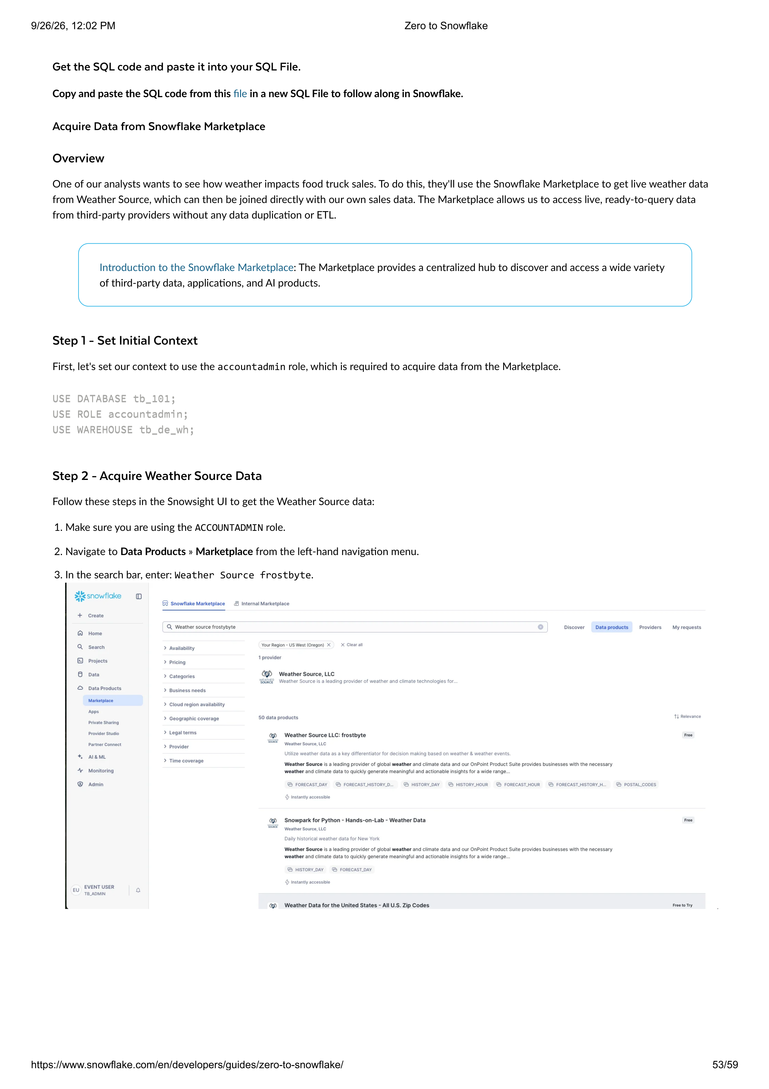
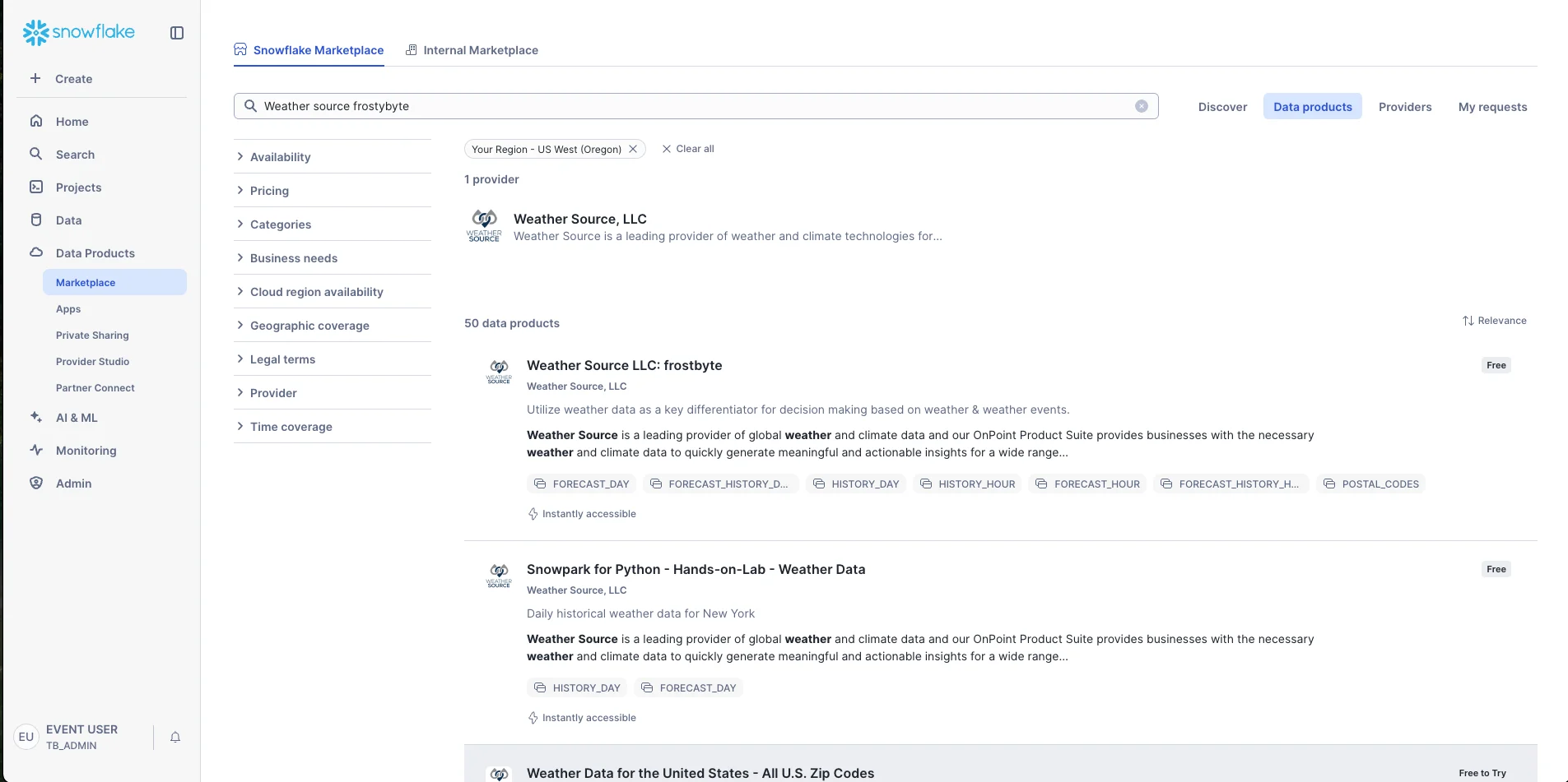
Get the SQL code and paste it into your SQL File.
Acquire Data from Snowflake Marketplace
Overview
Step 1 - Set Initial Context
Step 2 - Acquire Weather Source Data
Copy and paste the SQL code from this
file
in a new SQL File to follow along in Snowflake.
One of our analysts wants to see how weather impacts food truck sales. To do this, they'll use the Snowflake Marketplace to get live weather data
from Weather Source, which can then be joined directly with our own sales data. The Marketplace allows us to access live, ready-to-query data
from third-party providers without any data duplication or ETL.
Introduction to the Snowflake Marketplace
: The Marketplace provides a centralized hub to discover and access a wide variety
of third-party data, applications, and AI products.
First, let's set our context to use the
accountadmin
role, which is required to acquire data from the Marketplace.
USE DATABASE tb_101;
USE DATABASE tb_101;
USE ROLE accountadmin;
USE ROLE accountadmin;
USE WAREHOUSE tb_de_wh;
USE WAREHOUSE tb_de_wh;
Follow these steps in the Snowsight UI to get the Weather Source data:
1.
2.
3. In the search bar, enter:
Weather Source frostbyte
.
Make sure you are using the
ACCOUNTADMIN
role.
Navigate to
Data Products
»
Marketplace
from the left-hand navigation menu.
9/26/26, 12:02 PM
Zero to Snowflake
https://www.snowflake.com/en/developers/guides/zero-to-snowflake/
53/59
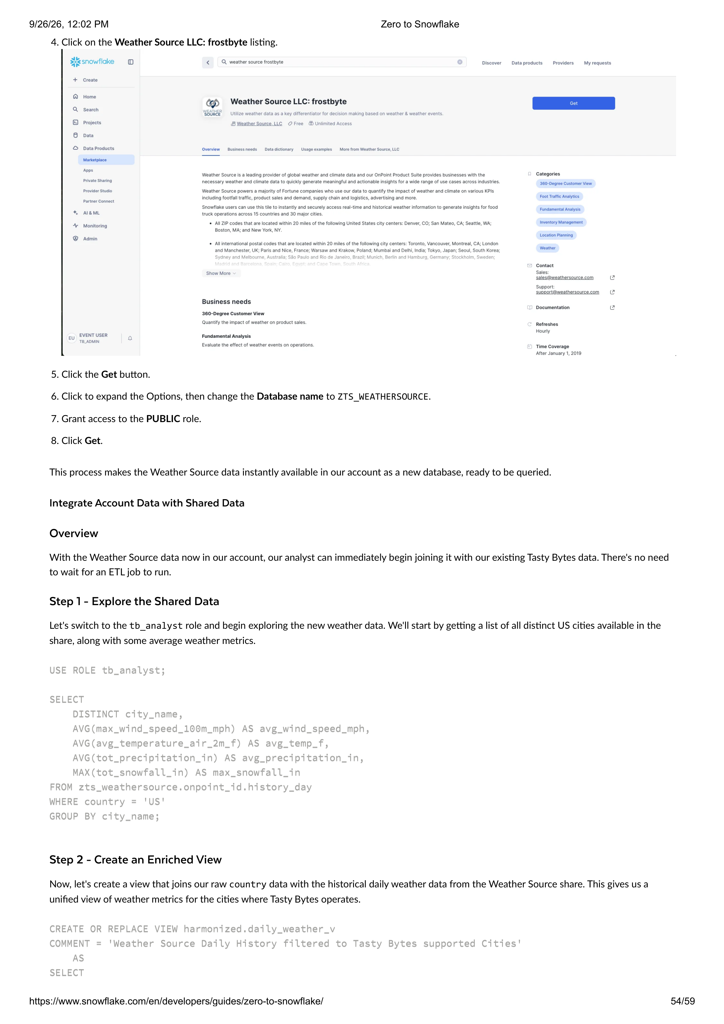
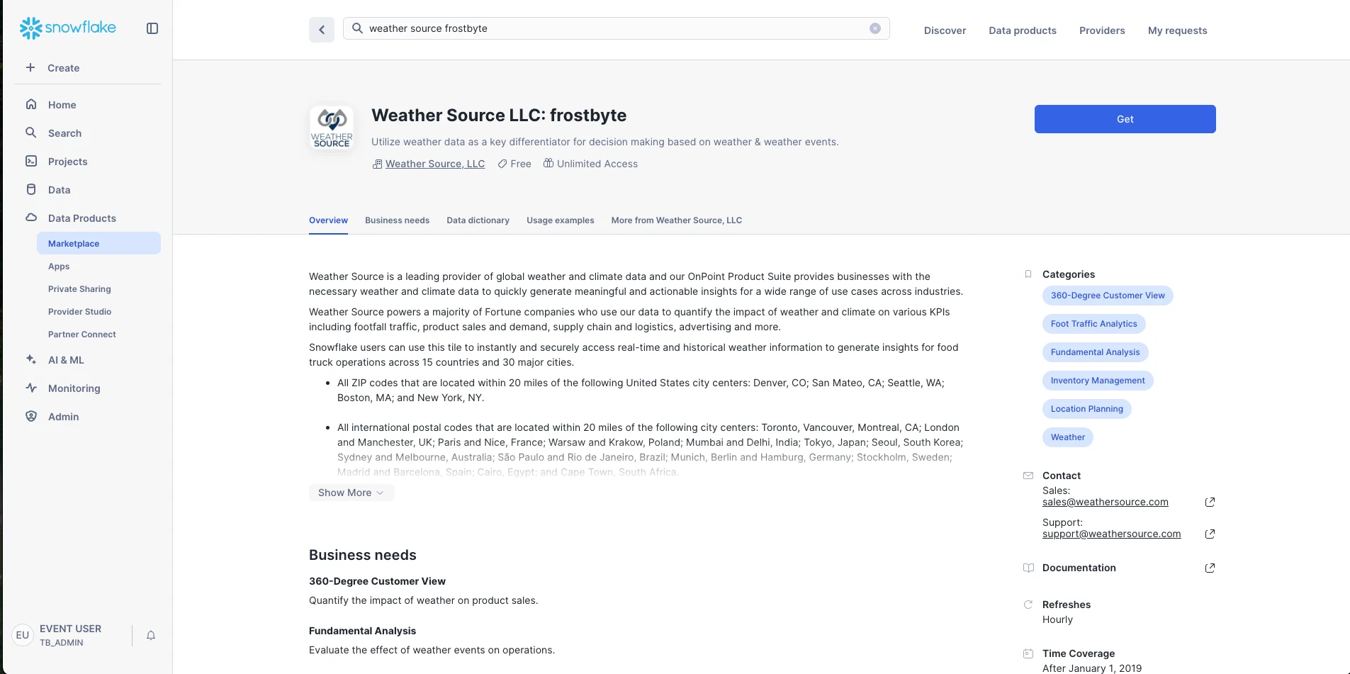
Integrate Account Data with Shared Data
Overview
Step 1 - Explore the Shared Data
Step 2 - Create an Enriched View
4. Click on the
Weather Source LLC: frostbyte
listing.
5.
6.
7.
8.
Click the
Get
button.
Click to expand the Options, then change the
Database name
to
ZTS_WEATHERSOURCE
.
Grant access to the
PUBLIC
role.
Click
Get
.
This process makes the Weather Source data instantly available in our account as a new database, ready to be queried.
With the Weather Source data now in our account, our analyst can immediately begin joining it with our existing Tasty Bytes data. There's no need
to wait for an ETL job to run.
Let's switch to the
tb_analyst
role and begin exploring the new weather data. We'll start by getting a list of all distinct US cities available in the
share, along with some average weather metrics.
USE ROLE tb_analyst;
USE ROLE tb_analyst;
SELECT
SELECT
DISTINCT city_name,
DISTINCT city_name,
AVG(max_wind_speed_100m_mph) AS avg_wind_speed_mph,
AVG(max_wind_speed_100m_mph) AS avg_wind_speed_mph,
AVG(avg_temperature_air_2m_f) AS avg_temp_f,
AVG(avg_temperature_air_2m_f) AS avg_temp_f,
AVG(tot_precipitation_in) AS avg_precipitation_in,
AVG(tot_precipitation_in) AS avg_precipitation_in,
MAX(tot_snowfall_in) AS max_snowfall_in
MAX(tot_snowfall_in) AS max_snowfall_in
FROM zts_weathersource.onpoint_id.history_day
FROM zts_weathersource.onpoint_id.history_day
WHERE country = 'US'
WHERE country = 'US'
GROUP BY city_name;
GROUP BY city_name;
Now, let's create a view that joins our raw
country
data with the historical daily weather data from the Weather Source share. This gives us a
unified view of weather metrics for the cities where Tasty Bytes operates.
CREATE OR REPLACE VIEW harmonized.daily_weather_v
CREATE OR REPLACE VIEW harmonized.daily_weather_v
COMMENT = 'Weather Source Daily History filtered to Tasty Bytes supported Cities'
COMMENT = 'Weather Source Daily History filtered to Tasty Bytes supported Cities'
AS
AS
SELECT
SELECT
9/26/26, 12:02 PM
Zero to Snowflake
https://www.snowflake.com/en/developers/guides/zero-to-snowflake/
54/59
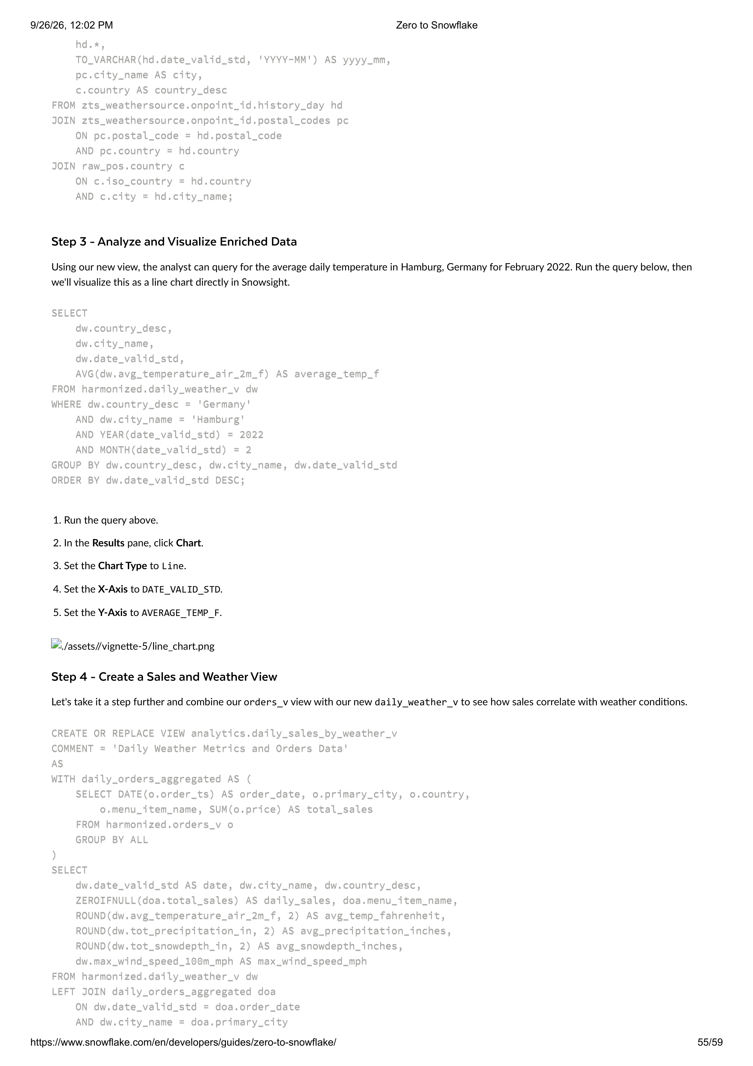

Step 3 - Analyze and Visualize Enriched Data
./assets//vignette-5/line_chart.png
Step 4 - Create a Sales and Weather View
hd.*,
hd.*,
TO_VARCHAR(hd.date_valid_std, 'YYYY-MM') AS yyyy_mm,
TO_VARCHAR(hd.date_valid_std, 'YYYY-MM') AS yyyy_mm,
pc.city_name AS city,
pc.city_name AS city,
c.country AS country_desc
c.country AS country_desc
FROM zts_weathersource.onpoint_id.history_day hd
FROM zts_weathersource.onpoint_id.history_day hd
JOIN zts_weathersource.onpoint_id.postal_codes pc
JOIN zts_weathersource.onpoint_id.postal_codes pc
ON pc.postal_code = hd.postal_code
ON pc.postal_code = hd.postal_code
AND pc.country = hd.country
AND pc.country = hd.country
JOIN raw_pos.country c
JOIN raw_pos.country c
ON c.iso_country = hd.country
ON c.iso_country = hd.country
AND c.city = hd.city_name;
AND c.city = hd.city_name;
Using our new view, the analyst can query for the average daily temperature in Hamburg, Germany for February 2022. Run the query below, then
we'll visualize this as a line chart directly in Snowsight.
SELECT
SELECT
dw.country_desc,
dw.country_desc,
dw.city_name,
dw.city_name,
dw.date_valid_std,
dw.date_valid_std,
AVG(dw.avg_temperature_air_2m_f) AS average_temp_f
AVG(dw.avg_temperature_air_2m_f) AS average_temp_f
FROM harmonized.daily_weather_v dw
FROM harmonized.daily_weather_v dw
WHERE dw.country_desc = 'Germany'
WHERE dw.country_desc = 'Germany'
AND dw.city_name = 'Hamburg'
AND dw.city_name = 'Hamburg'
AND YEAR(date_valid_std) = 2022
AND YEAR(date_valid_std) = 2022
AND MONTH(date_valid_std) = 2
AND MONTH(date_valid_std) = 2
GROUP BY dw.country_desc, dw.city_name, dw.date_valid_std
GROUP BY dw.country_desc, dw.city_name, dw.date_valid_std
ORDER BY dw.date_valid_std DESC;
ORDER BY dw.date_valid_std DESC;
1. Run the query above.
2. In the
Results
pane, click
Chart
.
3. Set the
Chart Type
to
Line
.
4. Set the
X-Axis
to
DATE_VALID_STD
.
5. Set the
Y-Axis
to
AVERAGE_TEMP_F
.
Let's take it a step further and combine our
orders_v
view with our new
daily_weather_v
to see how sales correlate with weather conditions.
CREATE OR REPLACE VIEW analytics.daily_sales_by_weather_v
CREATE OR REPLACE VIEW analytics.daily_sales_by_weather_v
COMMENT = 'Daily Weather Metrics and Orders Data'
COMMENT = 'Daily Weather Metrics and Orders Data'
AS
AS
WITH daily_orders_aggregated AS (
WITH daily_orders_aggregated AS (
SELECT DATE(o.order_ts) AS order_date, o.primary_city, o.country,
SELECT DATE(o.order_ts) AS order_date, o.primary_city, o.country,
o.menu_item_name, SUM(o.price) AS total_sales
o.menu_item_name, SUM(o.price) AS total_sales
FROM harmonized.orders_v o
FROM harmonized.orders_v o
GROUP BY ALL
GROUP BY ALL
)
SELECT
SELECT
dw.date_valid_std AS date, dw.city_name, dw.country_desc,
dw.date_valid_std AS date, dw.city_name, dw.country_desc,
ZEROIFNULL(doa.total_sales) AS daily_sales, doa.menu_item_name,
ZEROIFNULL(doa.total_sales) AS daily_sales, doa.menu_item_name,
ROUND(dw.avg_temperature_air_2m_f, 2) AS avg_temp_fahrenheit,
ROUND(dw.avg_temperature_air_2m_f, 2) AS avg_temp_fahrenheit,
ROUND(dw.tot_precipitation_in, 2) AS avg_precipitation_inches,
ROUND(dw.tot_precipitation_in, 2) AS avg_precipitation_inches,
ROUND(dw.tot_snowdepth_in, 2) AS avg_snowdepth_inches,
ROUND(dw.tot_snowdepth_in, 2) AS avg_snowdepth_inches,
dw.max_wind_speed_100m_mph AS max_wind_speed_mph
dw.max_wind_speed_100m_mph AS max_wind_speed_mph
FROM harmonized.daily_weather_v dw
FROM harmonized.daily_weather_v dw
LEFT JOIN daily_orders_aggregated doa
LEFT JOIN daily_orders_aggregated doa
ON dw.date_valid_std = doa.order_date
ON dw.date_valid_std = doa.order_date
AND dw.city_name = doa.primary_city
AND dw.city_name = doa.primary_city
9/26/26, 12:02 PM
Zero to Snowflake
https://www.snowflake.com/en/developers/guides/zero-to-snowflake/
55/59
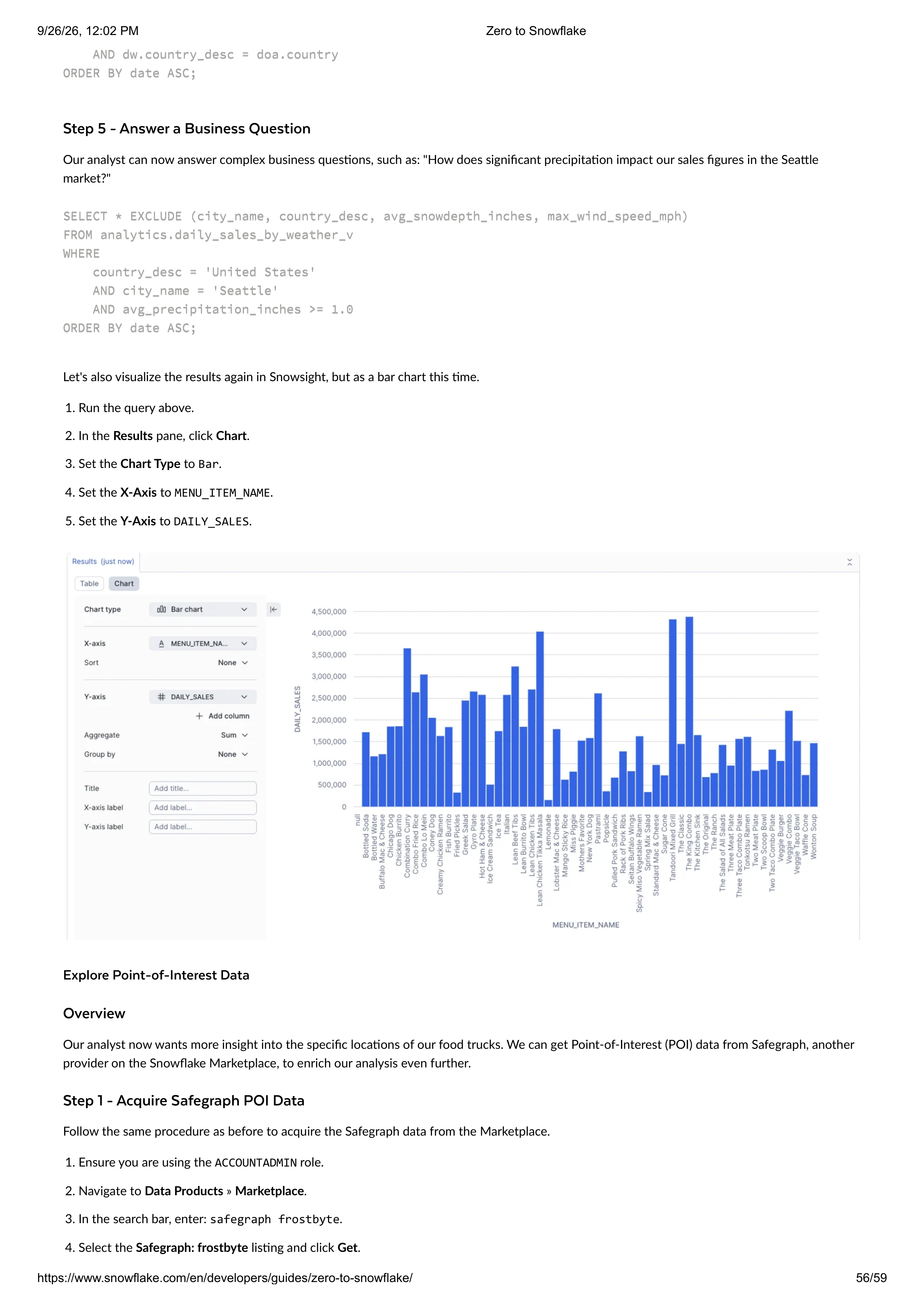
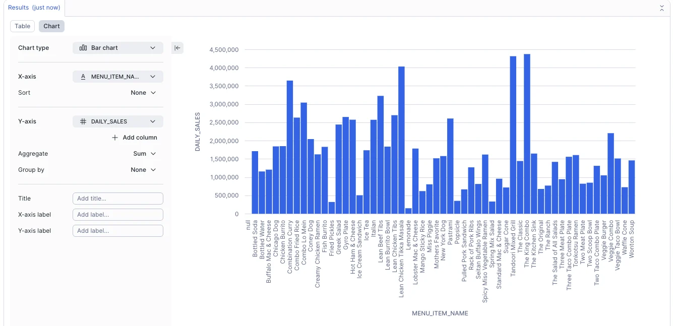
Step 5 - Answer a Business Question
Explore Point-of-Interest Data
Overview
Step 1 - Acquire Safegraph POI Data
AND dw.country_desc = doa.country
AND dw.country_desc = doa.country
ORDER BY date ASC;
ORDER BY date ASC;
Our analyst can now answer complex business questions, such as: "How does significant precipitation impact our sales figures in the Seattle
market?"
SELECT * EXCLUDE (city_name, country_desc, avg_snowdepth_inches, max_wind_speed_mph)
SELECT * EXCLUDE (city_name, country_desc, avg_snowdepth_inches, max_wind_speed_mph)
FROM analytics.daily_sales_by_weather_v
FROM analytics.daily_sales_by_weather_v
WHERE
WHERE
country_desc = 'United States'
country_desc = 'United States'
AND city_name = 'Seattle'
AND city_name = 'Seattle'
AND avg_precipitation_inches >= 1.0
AND avg_precipitation_inches >= 1.0
ORDER BY date ASC;
ORDER BY date ASC;
Let's also visualize the results again in Snowsight, but as a bar chart this time.
1. Run the query above.
2. In the
Results
pane, click
Chart
.
3. Set the
Chart Type
to
Bar
.
4. Set the
X-Axis
to
MENU_ITEM_NAME
.
5. Set the
Y-Axis
to
DAILY_SALES
.
Our analyst now wants more insight into the specific locations of our food trucks. We can get Point-of-Interest (POI) data from Safegraph, another
provider on the Snowflake Marketplace, to enrich our analysis even further.
Follow the same procedure as before to acquire the Safegraph data from the Marketplace.
1. Ensure you are using the
ACCOUNTADMIN
role.
2. Navigate to
Data Products
»
Marketplace
.
3. In the search bar, enter:
safegraph frostbyte
.
4. Select the
Safegraph: frostbyte
listing and click
Get
.
9/26/26, 12:02 PM
Zero to Snowflake
https://www.snowflake.com/en/developers/guides/zero-to-snowflake/
56/59
Step 2 - Create a POI View
Step 3 - Combine POI and Weather Data
Step 4 - Analyze Brand Resilience to Weather
5. Click to expand the Options, then set the
Database name
to
ZTS_SAFEGRAPH
.
6. Grant access to the
PUBLIC
role.
7. Click
Get
.
Let's create a view that joins our internal
location
data with the Safegraph POI data.
CREATE OR REPLACE VIEW harmonized.tastybytes_poi_v
CREATE OR REPLACE VIEW harmonized.tastybytes_poi_v
AS
AS
SELECT
SELECT
l.location_id, sg.postal_code, sg.country, sg.city, sg.iso_country_code,
l.location_id, sg.postal_code, sg.country, sg.city, sg.iso_country_code,
sg.location_name, sg.top_category, sg.category_tags,
sg.location_name, sg.top_category, sg.category_tags,
sg.includes_parking_lot, sg.open_hours
sg.includes_parking_lot, sg.open_hours
FROM raw_pos.location l
FROM raw_pos.location l
JOIN zts_safegraph.public.frostbyte_tb_safegraph_s sg
JOIN zts_safegraph.public.frostbyte_tb_safegraph_s sg
ON l.location_id = sg.location_id
ON l.location_id = sg.location_id
AND l.iso_country_code = sg.iso_country_code;
AND l.iso_country_code = sg.iso_country_code;
Now we can combine all three datasets: our internal data, the weather data, and the POI data. Let's find our top 3 windiest truck locations in the US
in 2022.
SELECT TOP 3
SELECT TOP 3
p.location_id, p.city, p.postal_code,
p.location_id, p.city, p.postal_code,
AVG(hd.max_wind_speed_100m_mph) AS average_wind_speed
AVG(hd.max_wind_speed_100m_mph) AS average_wind_speed
FROM harmonized.tastybytes_poi_v AS p
FROM harmonized.tastybytes_poi_v AS p
JOIN zts_weathersource.onpoint_id.history_day AS hd
JOIN zts_weathersource.onpoint_id.history_day AS hd
ON p.postal_code = hd.postal_code
ON p.postal_code = hd.postal_code
WHERE
WHERE
p.country = 'United States'
p.country = 'United States'
AND YEAR(hd.date_valid_std) = 2022
AND YEAR(hd.date_valid_std) = 2022
GROUP BY p.location_id, p.city, p.postal_code
GROUP BY p.location_id, p.city, p.postal_code
ORDER BY average_wind_speed DESC;
ORDER BY average_wind_speed DESC;
Finally, let's conduct a more complex analysis to determine brand resilience. We'll use a Common Table Expression (CTE) to first find the windiest
locations, and then compare sales on "calm" vs. "windy" days for each truck brand at those locations. This can help inform operational decisions, like
offering "Windy Day" promotions for brands that are less resilient.
WITH TopWindiestLocations AS (
WITH TopWindiestLocations AS (
SELECT TOP 3
SELECT TOP 3
p.location_id
p.location_id
FROM harmonized.tastybytes_poi_v AS p
FROM harmonized.tastybytes_poi_v AS p
JOIN zts_weathersource.onpoint_id.history_day AS hd ON p.postal_code = hd.postal_code
JOIN zts_weathersource.onpoint_id.history_day AS hd ON p.postal_code = hd.postal_code
WHERE p.country = 'United States' AND YEAR(hd.date_valid_std) = 2022
WHERE p.country = 'United States' AND YEAR(hd.date_valid_std) = 2022
GROUP BY p.location_id, p.city, p.postal_code
GROUP BY p.location_id, p.city, p.postal_code
ORDER BY AVG(hd.max_wind_speed_100m_mph) DESC
ORDER BY AVG(hd.max_wind_speed_100m_mph) DESC
)
SELECT
SELECT
o.truck_brand_name,
o.truck_brand_name,
ROUND(AVG(CASE WHEN hd.max_wind_speed_100m_mph <= 20 THEN o.order_total END), 2) AS avg_sales_calm_days,
ROUND(AVG(CASE WHEN hd.max_wind_speed_100m_mph <= 20 THEN o.order_total END), 2) AS avg_sales_calm_days,
ZEROIFNULL(ROUND(AVG(CASE WHEN hd.max_wind_speed_100m_mph > 20 THEN o.order_total END), 2)) AS avg_sales_w
ZEROIFNULL(ROUND(AVG(CASE WHEN hd.max_wind_speed_100m_mph > 20 THEN o.order_total END), 2)) AS avg_sales_w
FROM analytics.orders_v AS o
FROM analytics.orders_v AS o
JOIN zts_weathersource.onpoint_id.history_day AS hd
JOIN zts_weathersource.onpoint_id.history_day AS hd
ON o.primary_city = hd.city_name AND DATE(o.order_ts) = hd.date_valid_std
ON o.primary_city = hd.city_name AND DATE(o.order_ts) = hd.date_valid_std
WHERE o.location_id IN (SELECT location_id FROM TopWindiestLocations)
WHERE o.location_id IN (SELECT location_id FROM TopWindiestLocations)
GROUP BY o.truck_brand_name
GROUP BY o.truck_brand_name
ORDER BY o.truck_brand_name;
ORDER BY o.truck_brand_name;
9/26/26, 12:02 PM
Zero to Snowflake
https://www.snowflake.com/en/developers/guides/zero-to-snowflake/
57/59

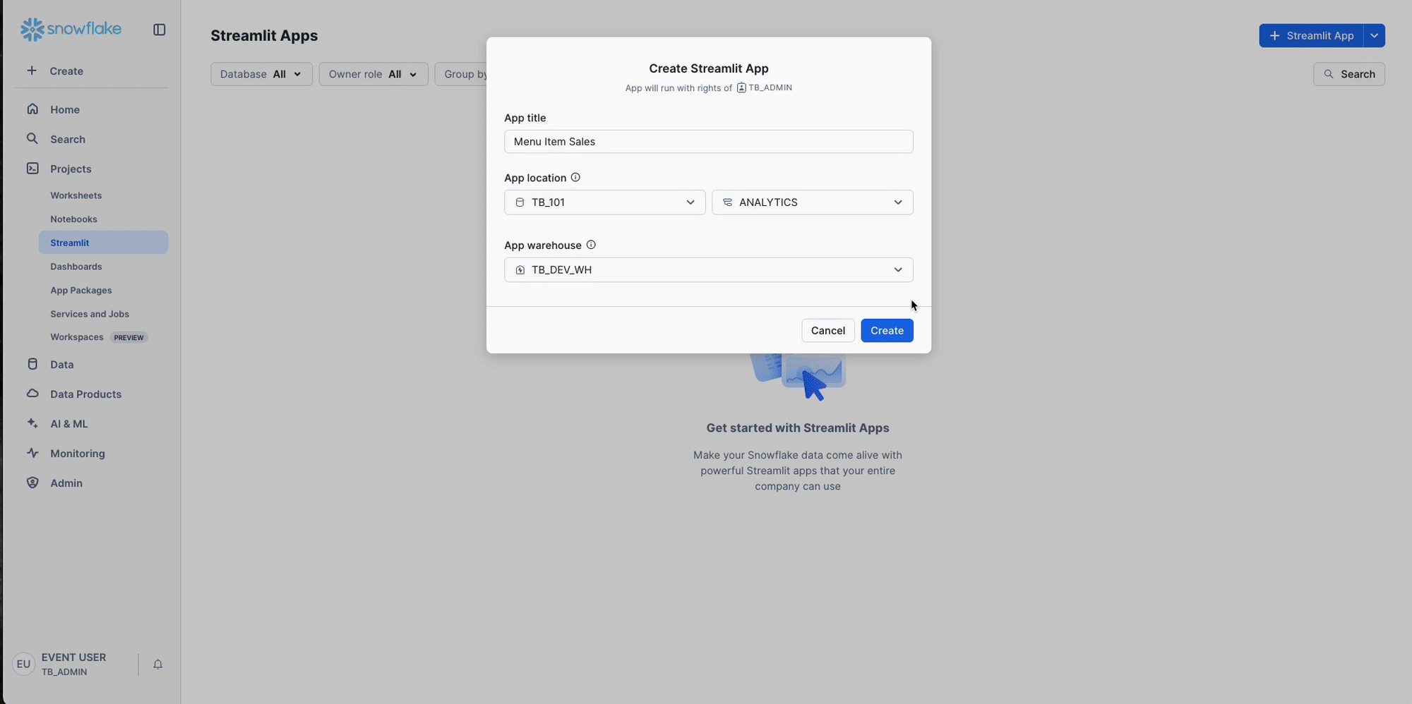
Introduction to Streamlit in Snowflake
Step 1 - Create Streamlit App
Conclusion and Resources
Streamlit is an open-source Python library designed for easily creating and sharing web applications for machine learning and data science. It allows
for the rapid development and deployment of data-driven apps.
Streamlit in Snowflake empowers developers to securely build, deploy, and share applications directly within Snowflake. This integration allows you
to build apps that process and utilize data stored in Snowflake without the need of moving the data or application code to an external system.
Let's create our first Streamlit app, an app that will display and chart sales data for each menu item in Japan for February 2022.
1.
2.
3.
4.
5.
First, navigate to
Projects
»
Streamlit
, then click on the blue '+ Streamlit App' button in the top right to create a new app.
Enter these values in the 'Create Streamlit App' pop-up:
App title: Menu Item Sales
App location:
Database: tb_101
Schema: Analytics
App warehouse: tb_dev_wh
Now click 'Create'. When the app first loads, you'll see a sample app on the right pane and the app's code in the editor pane to the left.
Select all of the code and remove it.
Next copy + paste this
code
in the blank editor window, then click 'Run' in the top right.
9/26/26, 12:02 PM
Zero to Snowflake
https://www.snowflake.com/en/developers/guides/zero-to-snowflake/
58/59
Overview
What You Learned
Resources
Congratulations! You have successfully completed the entire Tasty Bytes - Zero to Snowflake journey.
You have now built and configured warehouses, cloned and transformed data, recovered a dropped table with Time Travel, and built an automated
data pipeline for semi-structured data. You've also unlocked insights using AI by generating analysis with simple AISQL functions and accelerating
your workflow with Snowflake Copilot. Furthermore, you have implemented a robust governance framework with roles and policies and seamlessly
enriched your own data with live datasets from the Snowflake Marketplace.
If you would like to re-run this Quickstart, please run the complete
RESET
script located at the bottom of your SQL file.
Warehousing and Performance:
How to create, manage, and scale virtual warehouses, and leverage Snowflake's results cache.
Data Transformation:
How to use Zero-Copy Cloning for safe development, transform data, and instantly recover from errors using Time Travel
and
UNDROP
.
Data Pipelines:
How to ingest data from external stages, process semi-structured
VARIANT
data, and build automated ELT pipelines with
Dynamic Tables.
Snowflake Cortex AI
How to leverage Snowflake Cortex AI to build a customer analytics platform.
Data Governance:
How to implement a security framework using Role-Based Access Control, automated PII classification, tag-based Data
Masking, and Row Access Policies.
Data Collaboration:
How to discover and acquire live, third-party datasets from the Snowflake Marketplace and seamlessly join them with your
own data to generate new insights.
Virtual Warehouses & Settings
Resource Monitors
Budgets
Universal Search
Ingestion from External Stage
Semi-Structured Data
Dynamic Tables
Roles & Access Control
Tag-Based Classification
Column Level Security with Masking Policies
Row Level Security with Row Access Policies
Data Metric Functions
Trust Center
Data Sharing
Snowflake Cortex Playground
AI SQL Functions in Snowflake Cortex
Snowflake Cortex Search Overview
Snowflake Cortex Analyst
Updated Dec 11, 2025
This content is provided as is, and is not maintained on an ongoing basis. It may be out of date with current Snowflake instances
Product
Platform
Snowflake CoWork
Data Engineering
Analytics
AI
Applications & Collaboration
Pricing
Support
Support
Priority Support
Status
Industries
Advertising, Media & Entertainment
Financial Services
Healthcare & Life Sciences
Manufacturing
Public Sector
Retail & Consumer Goods
Telecom
Technology
Company
About Snowflake
Leadership & Board
Careers
Investor Relations
Trust Center
Brand Guidelines
Contact
Newsroom
Environmental, Social & Governance
Snowflake Ventures
End Data Disparity
Snowflake Summit 26
Learn
Resource Library
Live Demos
Fundamentals
Training
Certifications
Snowflake University
Developer Guides
Documentation
Data Governance
Subscribe to our monthly newsletter
Stay up to date on Snowflake’s latest products, expert insights and resources—right in your inbox!
© 2026 Snowflake Inc. All Rights Reserved
Privacy Policy
Site Terms
Communication Preferences
Cookies Settings
Do Not Share My Personal Information
Legal
9/26/26, 12:02 PM
Zero to Snowflake
https://www.snowflake.com/en/developers/guides/zero-to-snowflake/
59/59