
Compute-Optimal
Quantization-Aware Training
Aleksandr Dremov
∗
,
David Grangier
,
Angelos Katharopoulos
,
Awni Hannun
Apple
Quantization-aware training (QAT) is a leading technique for improving the accuracy of quantized neural networks. Previ-
ous work has shown that decomposing training into a full-precision (FP) phase followed by a QAT phase yields superior
accuracy compared to QAT alone. However, the optimal allocation of compute between the FP and QAT phases remains
unclear. We conduct extensive experiments with various compute budgets, QAT bit widths, and model sizes from 86.0M
to 2.2B to investigate how different QAT durations impact final performance.
We demonstrate that, contrary to previous
findings,
the loss-optimal ratio of QAT to FP training increases with the total amount of compute.
Moreover,
the opti-
mal fraction can be accurately predicted for a wide range of model sizes and quantization widths using the tokens-per-
parameter-byte statistic. From experimental data, we derive a loss scaling law that predicts both optimal QAT ratios and fi-
nal model performance across different QAT/FP compute allocation strategies and QAT bit widths. We use the scaling law
to make further predictions, which we verify experimentally, including which QAT bit width is optimal under a given mem-
ory constraint and how QAT accuracy with different bit widths compares to full-precision model accuracy.
Additionally,
we propose a novel cooldown and QAT fusion approach that performs learning rate decay jointly with quantization-aware
training, eliminating redundant full-precision model updates and achieving significant compute savings.
These findings
provide practical insights into efficient QAT planning and enable the training of higher-quality quantized models with the
same compute budget.
Correspondence:
{alexdremov,
grangier,
a_katharopoulos,
awni}@apple.com
Date:
February 27, 2026
1
Introduction
As
Large
Language
Models
(LLMs)
grow
in
size
and
on-device
applications
gain
traction
(
Xu
et
al.
,
2024
),
significant attention has been devoted to reducing inference costs via model compression (
Frantar et al.
,
2022
;
Lin
et
al.
,
2024
;
Ma
et
al.
,
2023
).
One
state-of-the-art
method
is
quantization-aware
training
(QAT)
(
Chen
et
al.
,
2025a
;
Lin
et
al.
,
2024
;
Liu
et
al.
,
2025
;
Jacob
et
al.
,
2018
).
To
adapt
the
model
to
the
loss
of
numerical
precision,
QAT
incorporates
quantization
directly
into
the
model
training
process.
It
has
been
shown
that
QAT
outperforms
post-training
quantization
(PTQ)
(
Xiao
et
al.
,
2023
;
Banner
et
al.
,
2019
),
where
quantization
is
applied
after
training
is
completed.
Moreover,
Liu
et
al.
(
2025
)
demonstrated
that
the
best
accuracy
is
achieved
when
a
QAT
phase
follows
a
full-precision
(FP)
training
phase.
For
models
designed
for
on-device
use,
the
QAT
stage
is
an
important
part
of
the
training
process
and
is
usually
planned
in
advance.
As
model
sizes
grow
and
deployment
constraints
tighten,
practitioners
face
a
critical
resource
allocation
problem:
given
a
fixed
compute
budget,
how
should
training
time
be
divided
between
full-precision
pretraining
and
quantization-aware
training?
This
decision
directly impacts both model quality and deployment efficiency, yet existing guidelines assume fixed allocation
ratios
regardless
of
scale.
As
motivation,
we
note
that
Kumar
et
al.
(
2025
)
demonstrated
that
the
error
introduced
by
post-training
quantization
grows
with
the
size
of
the
pretraining
data,
which
can
actually
make
additional
pretraining
harmful.
Intuitively,
analogous
to
PTQ,
having
a
longer
full-precision
stage
* Work done at Apple during internship while studying at École Polytechnique Fédérale de Lausanne (EPFL),
aleksandr.dremov@epfl.ch
.
1
arXiv:2509.22935v2 [cs.LG] 26 Feb 2026

should
make
subsequent
QAT
more
difficult.
While
Liu
et
al.
(
2025
)
showed
that
spending
10%
of
the
training
steps
on
QAT
is
optimal
for
some
setups,
the
authors
did
not
explore
how
this
proportion
varies
across
different
training
lengths
and
model
sizes.
In
this
work,
we
show
that
previous
conclusions
about
optimal
QAT
length
do
not
hold
with
an
increased
compute
budget.
Through
a
series
of
experiments
with
different
model
sizes
and
token
counts,
we
demon-
strate
that
the
optimal
fraction
of
QAT
compared
to
the
total
training
length
increases
with
the
total
compute
budget.
This
optimum
can
be
accurately
predicted
for
a
wide
range
of
setups
using
the
tokens-
per-parameter-byte
statistic.
Additionally, we propose a loss scaling law as a function of model parameter
count
(
N
),
token
count
spent
on
full-precision
training
(
D
fp
),
token
count
spent
on
QAT
(
D
qat
),
and
QAT
bit-width
(
B
).
The
fitted
law
accurately
captures
the
growth
of
the
optimal
QAT
fraction
with
compute
scale.
The
key
contributions
of
this
study
are:
•
Unlike
previously
assumed,
we
find
that
the
optimal
fraction
allocated
for
QAT
increases
with
the
growth
of
the
tokens-per-parameter-byte
statistic.
This
finding
allows
higher-quality
quantized
models
to
be
achieved
with
the
same
initial
compute
budget
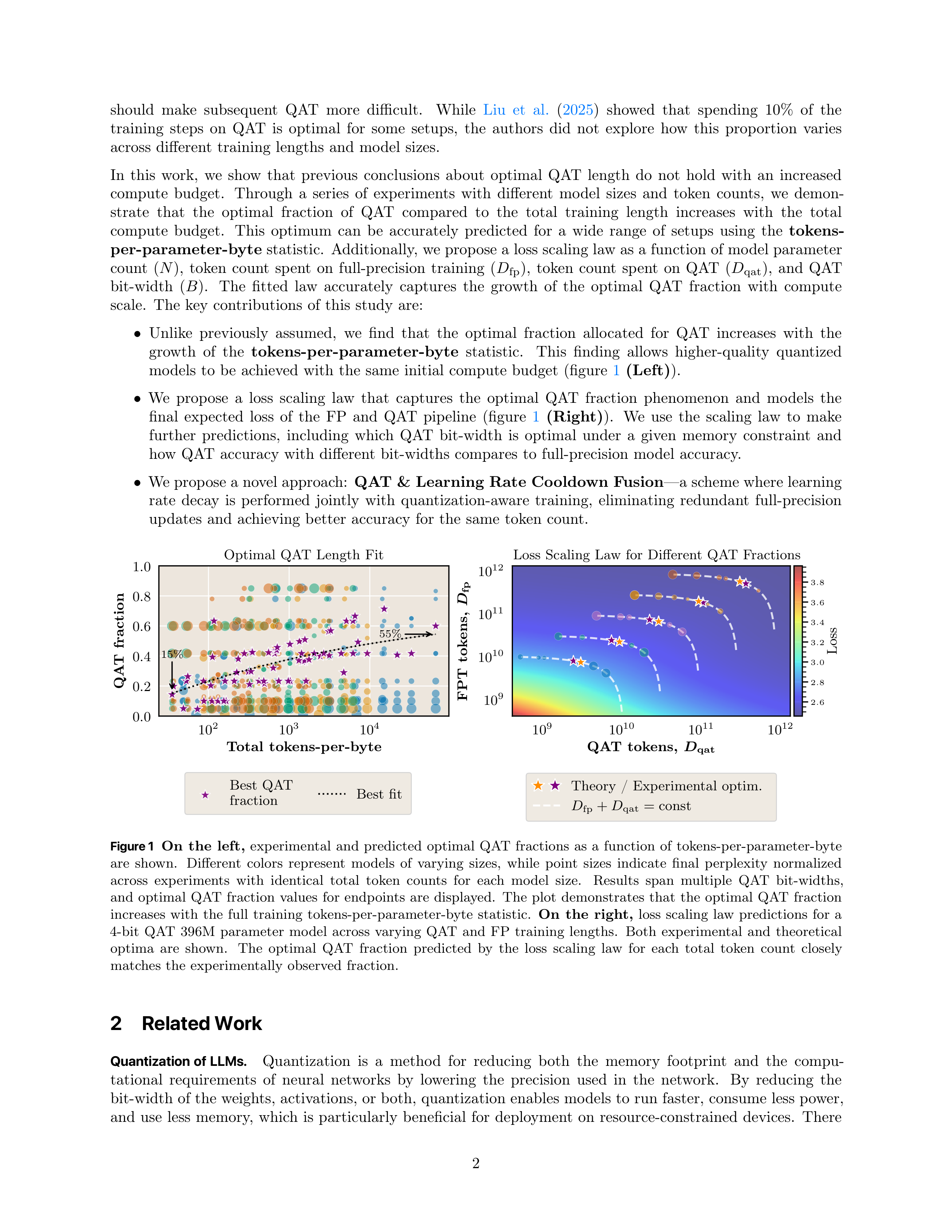
(figure
1
(Left)
).
•
We
propose
a
loss
scaling
law
that
captures
the
optimal
QAT
fraction
phenomenon
and
models
the
final
expected
loss
of
the
FP
and
QAT
pipeline
(figure
1
(Right)
).
We
use
the
scaling
law
to
make
further
predictions,
including
which
QAT
bit-width
is
optimal
under
a
given
memory
constraint
and
how
QAT
accuracy
with
different
bit-widths
compares
to
full-precision
model
accuracy.
•
We propose a novel approach:
QAT
&
Learning
Rate
Cooldown
Fusion
—a scheme where learning
rate
decay
is
performed
jointly
with
quantization-aware
training,
eliminating
redundant
full-precision
updates
and
achieving
better
accuracy
for
the
same
token
count.
10
2
10
3
10
4
Total
tokens-per-byte
0
.
0
0
.
2
0
.
4
0
.
6
0
.
8
1
.
0
QAT
fraction
15%
55%
Optimal
QAT
Length
Fit
Best
QAT
fraction
Best
fit
10
9
10
10
10
11
10
12
QAT
tokens,
D
qat
10
9
10
10
10
11
10
12
FPT
tokens,
D
fp
Loss
Scaling
Law
for
Different
QAT
Fractions
Theory
/
Experimental
optim.
D
fp
+
D
qat
=
const
2
.
6
2
.
8
3
.
0
3
.
2
3
.
4
3
.
6
3
.
8
Loss
Figure 1
On
the
left,
experimental
and
predicted
optimal
QAT
fractions
as
a
function
of
tokens-per-parameter-byte
are
shown.
Different
colors
represent
models
of
varying
sizes,
while
point
sizes
indicate
final
perplexity
normalized
across
experiments
with
identical
total
token
counts
for
each
model
size.
Results
span
multiple
QAT
bit-widths,
and
optimal
QAT
fraction
values
for
endpoints
are
displayed.
The
plot
demonstrates
that
the
optimal
QAT
fraction
increases
with
the
full
training
tokens-per-parameter-byte
statistic.
On
the
right,
loss
scaling
law
predictions
for
a
4-bit
QAT
396M
parameter
model
across
varying
QAT
and
FP
training
lengths.
Both
experimental
and
theoretical
optima
are
shown.
The
optimal
QAT
fraction
predicted
by
the
loss
scaling
law
for
each
total
token
count
closely
matches
the
experimentally
observed
fraction.
2
Related Work
Quantization of LLMs.
Quantization
is
a
method
for
reducing
both
the
memory
footprint
and
the
compu-
tational
requirements
of
neural
networks
by
lowering
the
precision
used
in
the
network.
By
reducing
the
bit-width
of
the
weights,
activations,
or
both,
quantization
enables
models
to
run
faster,
consume
less
power,
and
use
less
memory,
which
is
particularly
beneficial
for
deployment
on
resource-constrained
devices.
There
2
are
different
quantization
techniques,
including
post-training
quantization
(PTQ)
(
Xiao
et
al.
,
2023
;
Banner
et
al.
,
2019
)
—
methods
that
transform
a
model
after
training
has
been
completed
and
usually
require
mini-
mal additional computational usage.
Another group of methods is quantization-aware training (QAT) (
Chen
et
al.
,
2025a
;
Lin
et
al.
,
2024
;
Liu
et
al.
,
2025
;
Jacob
et
al.
,
2018
),
which
quantizes
a
model
during
training,
allowing
the
model
to
better
adapt
to
precision
loss.
As
quantization
operations
are
non-differentiable,
train-
ing relies on gradient approximations such as the straight-through estimator (
Bengio et al.
,
2013
).
In contrast
to
PTQ,
QAT
requires
more
computation,
as
effectively
the
full
model
is
trained
with
added
quantization-
related
operations.
In
this
work,
we
focus
on
QAT,
as
it
is
the
method
most
commonly
used
in
practice
to
obtain
high-quality
quantized
models.
Loss Scaling Laws.
Multiple
works
have
previously
addressed
the
problem
of
predicting
final
model
loss
(
L
)
as
a
function
of
parameter
count
(
N
)
and
consumed
tokens
(
D
)
(
Bi
et
al.
,
2024
;
Hoffmann
et
al.
,
2022
;
Kaplan
et
al.
,
2020
).
The
Chinchilla
(
Hoffmann
et
al.
,
2022
)
loss
model
is
one
of
the
most
commonly
used:
L
(
N, D
) =
E
+
AN
−
α
+
CD
−
β
,
where
A
,
C
,
α
,
β
,
and
E
are
fitted
parameters.
Bi
et
al.
(
2024
)
expand
on
this
idea,
fitting
accuracy
as
a
function
of
used
non-embedding
FLOPs
(FLOP
estimation
of
model
inference
without
embedding
layer
calculations),
showing
that
such
an
approach
works
better
across
different
model
sizes.
Additionally,
they
show
that
scaling
laws
are
greatly
influenced
by
data
quality.
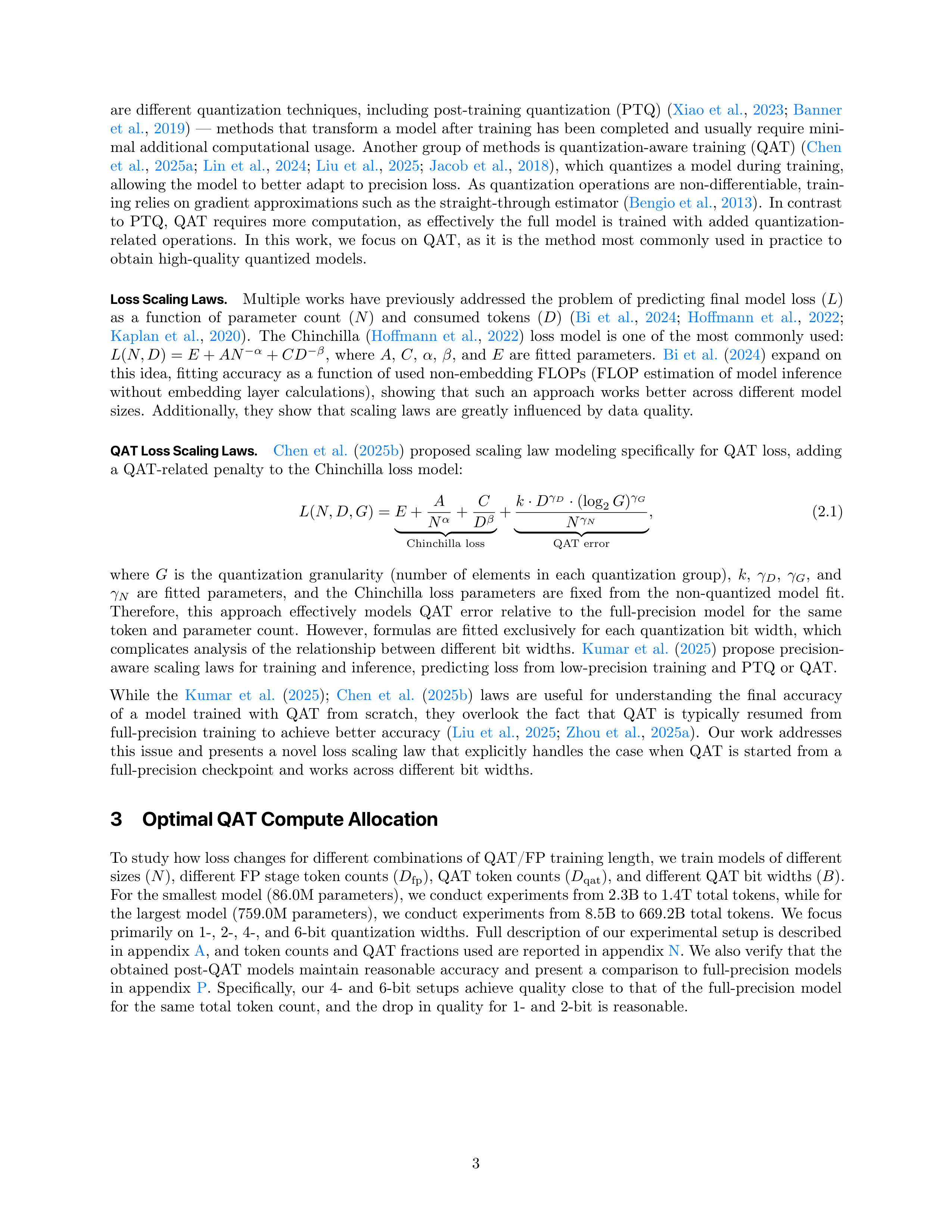
QAT Loss Scaling Laws.
Chen
et
al.
(
2025b
)
proposed
scaling
law
modeling
specifically
for
QAT
loss,
adding
a
QAT-related
penalty
to
the
Chinchilla
loss
model:
L
(
N, D, G
) =
E
+
A
N
α
+
C
D
β
|
{z
}
Chinchilla
loss
+
k
·
D
γ
D
·
(log
2
G
)
γ
G
N
γ
N
|
{z
}
QAT
error
,
(2.1)
where
G
is
the
quantization
granularity
(number
of
elements
in
each
quantization
group),
k
,
γ
D
,
γ
G
,
and
γ
N
are
fitted
parameters,
and
the
Chinchilla
loss
parameters
are
fixed
from
the
non-quantized
model
fit.
Therefore,
this
approach
effectively
models
QAT
error
relative
to
the
full-precision
model
for
the
same
token
and
parameter
count.
However,
formulas
are
fitted
exclusively
for
each
quantization
bit
width,
which
complicates
analysis
of
the
relationship
between
different
bit
widths.
Kumar
et
al.
(
2025
)
propose
precision-
aware
scaling
laws
for
training
and
inference,
predicting
loss
from
low-precision
training
and
PTQ
or
QAT.
While
the
Kumar
et
al.
(
2025
);
Chen
et
al.
(
2025b
)
laws
are
useful
for
understanding
the
final
accuracy
of
a
model
trained
with
QAT
from
scratch,
they
overlook
the
fact
that
QAT
is
typically
resumed
from
full-precision
training
to
achieve
better
accuracy
(
Liu
et
al.
,
2025
;
Zhou
et
al.
,
2025a
).
Our
work
addresses
this
issue
and
presents
a
novel
loss
scaling
law
that
explicitly
handles
the
case
when
QAT
is
started
from
a
full-precision
checkpoint
and
works
across
different
bit
widths.
3
Optimal QAT Compute Allocation
To study how loss changes for different combinations of QAT/FP training length, we train models of different
sizes (
N
), different FP stage token counts (
D
fp
), QAT token counts (
D
qat
), and different QAT bit widths (
B
).
For the smallest model (86.0M parameters), we conduct experiments from 2.3B to 1.4T total tokens, while for
the
largest
model
(759.0M
parameters),
we
conduct
experiments
from
8.5B
to
669.2B
total
tokens.
We
focus
primarily
on
1-,
2-,
4-,
and
6-bit
quantization
widths.
Full
description
of
our
experimental
setup
is
described
in appendix
A
, and token counts and QAT fractions used are reported in appendix
N
. We also verify that the
obtained
post-QAT
models
maintain
reasonable
accuracy
and
present
a
comparison
to
full-precision
models
in
appendix
P
.
Specifically,
our
4-
and
6-bit
setups
achieve
quality
close
to
that
of
the
full-precision
model
for
the
same
total
token
count,
and
the
drop
in
quality
for
1-
and
2-bit
is
reasonable.
3
The
main
objective
of
this
study
is
to
determine
the
optimal
QAT
fraction
f
∗
—the
fraction
of
the
token
count
that
should
be
dedicated
to
QAT
for
a
given
total
token
count.
This
can
be
formalized
as
the
following
minimization
problem:
D
∗
qat
(
N, D
total
, B
) =
arg min
D
qat
∈
N
,
D
qat
+
D
fp
=
D
total
L
(
N, D
fp
, D
qat
, B
)
,
f
∗
(
N, D
total
, B
) =
D
∗
qat
(
N, D
total
, B
)
D
total
,
where
L
(
N, D
fp
, D
qat
, B
)
is
the
final
loss
of
the
setup
with
D
fp
tokens
dedicated
to
FP
training
and
D
qat
tokens dedicated to
B
-bit QAT. Intuitively,
f
∗
expresses a trade-off.
On one hand, too few QAT steps do not
allow
the
quantized
model
to
adapt
to
reduced
precision.
On
the
other
hand,
too
many
QAT
steps
(at
the
expense
of
fewer
FP
steps)
should
also
lead
to
worse
loss
since
QAT
is
trained
with
gradient
approximations
for
quantization
operators,
which
introduces
biased
and
noisier
gradients.
Naturally,
a
trade-off
emerges,
suggesting
that
such
f
∗
should
be
well-defined.
3.1
Predicting the Optimal QAT Fraction
10
10
10
11
10
12
Total
tokens
10
10
10
11
QAT
tokens
Optima
Plot
(tokens)
10
2
10
3
Total
tokens-per-byte
10
1
10
2
10
3
QAT
tokens-per-byte
Optima
Plot
(tokens-per-byte)
B
1
2
4
6
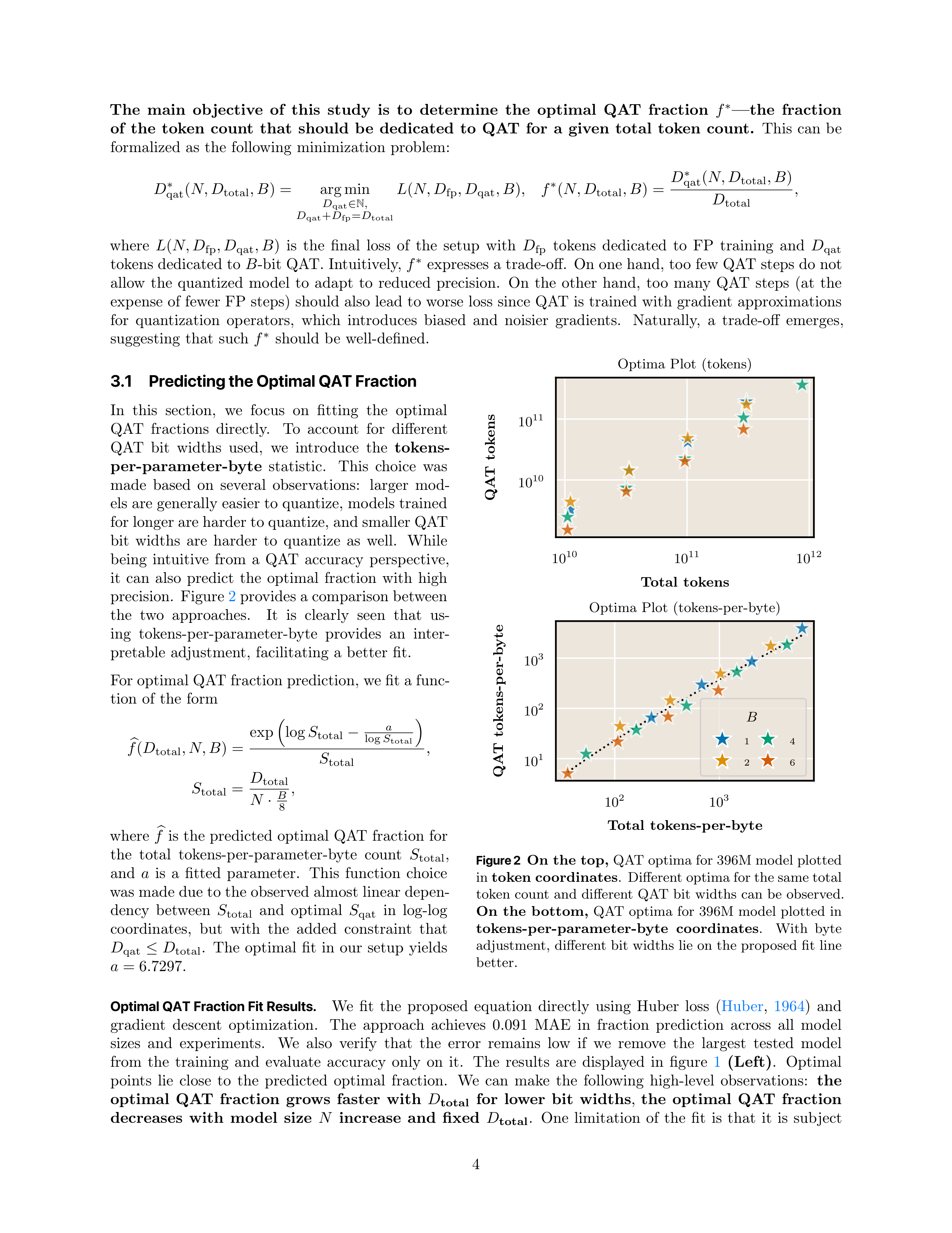
Figure 2
On
the
top,
QAT optima for 396M model plotted
in
token coordinates
.
Different optima for the same total
token
count
and
different
QAT
bit
widths
can
be
observed.
On
the
bottom,
QAT
optima
for
396M
model
plotted
in
tokens-per-parameter-byte
coordinates
.
With
byte
adjustment,
different
bit
widths
lie
on
the
proposed
fit
line
better.
In
this
section,
we
focus
on
fitting
the
optimal
QAT
fractions
directly.
To
account
for
different
QAT
bit
widths
used,
we
introduce
the
tokens-
per-parameter-byte
statistic.
This
choice
was
made
based
on
several
observations:
larger
mod-
els are generally easier to quantize, models trained
for longer are harder to quantize, and smaller QAT
bit
widths
are
harder
to
quantize
as
well.
While
being
intuitive
from
a
QAT
accuracy
perspective,
it
can
also
predict
the
optimal
fraction
with
high
precision.
Figure
2
provides a comparison between
the
two
approaches.
It
is
clearly
seen
that
us-
ing
tokens-per-parameter-byte
provides
an
inter-
pretable
adjustment,
facilitating
a
better
fit.
For optimal QAT fraction prediction, we fit a func-
tion
of
the
form
b
f
(
D
total
, N, B
) =
exp
log
S
total
−
a
log
S
total
S
total
,
S
total
=
D
total
N
·
B
8
,
where
b
f
is
the
predicted
optimal
QAT
fraction
for
the
total
tokens-per-parameter-byte
count
S
total
,
and
a
is
a
fitted
parameter.
This
function
choice
was made due to the observed almost linear depen-
dency
between
S
total
and
optimal
S
qat
in
log-log
coordinates,
but
with
the
added
constraint
that
D
qat
≤
D
total
.
The
optimal
fit
in
our
setup
yields
a
= 6
.
7297
.
Optimal QAT Fraction Fit Results.
We
fit
the
proposed
equation
directly
using
Huber
loss
(
Huber
,
1964
)
and
gradient
descent
optimization.
The
approach
achieves
0.091
MAE
in
fraction
prediction
across
all
model
sizes
and
experiments.
We
also
verify
that
the
error
remains
low
if
we
remove
the
largest
tested
model
from
the
training
and
evaluate
accuracy
only
on
it.
The
results
are
displayed
in
figure
1
(Left)
.
Optimal
points
lie
close
to
the
predicted
optimal
fraction.
We
can
make
the
following
high-level
observations:
the
optimal
QAT
fraction
grows
faster
with
D
total
for
lower
bit
widths
,
the
optimal
QAT
fraction
decreases
with
model
size
N
increase
and
fixed
D
total
.
One
limitation
of
the
fit
is
that
it
is
subject
4
to
the
granularity
of
the
selected
experiments—the
set
of
QAT
fractions
being
tested.
Also,
as
we
fit
only
optimal
points,
we
do
not
use
a
substantial
amount
of
non-optimal
data
points,
which
also
contain
valuable
information about loss behavior.
One way to utilize all available data is to model the loss scaling law explicitly
and
infer
optimal
QAT
fractions
from
it.
We
focus
on
this
in
section
3.2
.
Takeaway 1
Optimal
QAT
compute
allocation
fraction
is
not
stationary
but
grows
with
total
training
tokens-per-
parameter-byte
(
S
total
)
and
can
be
predicted
from
it.
3.2
Loss Scaling Law
As described in section
2
,
Chen et al.
(
2025b
) were able to fit a loss scaling law for QAT started from scratch
(
D
fp
= 0
).
We
extend
this
idea
by
making
the
loss
scaling
law
dependent
not
only
on
D
total
but
also
on
D
fp
,
D
qat
,
and
B
,
essentially
modeling
loss
for
different
QAT
fractions
and
bit-widths.
However,
we
do
not
follow
the
same
functional
form
as
that
proposed
by
Chen
et
al.
(
2025b
).
This
is
because
in
equation
2.1
,
the
QAT
penalty
overtakes
the
Chinchilla
loss
term
at
some
point
with
the
growth
of
token
count,
which
causes
the
limit
of
the
whole
expression
to
approach
infinity
as
D
total
→∞
.
This
does
not
align
with
the
expected
loss
decrease
as
token
count
grows
and
will
hinder
making
any
predictions
from
the
scaling
law
in
the
future.
We
propose
a
loss
model
in
the
form
of
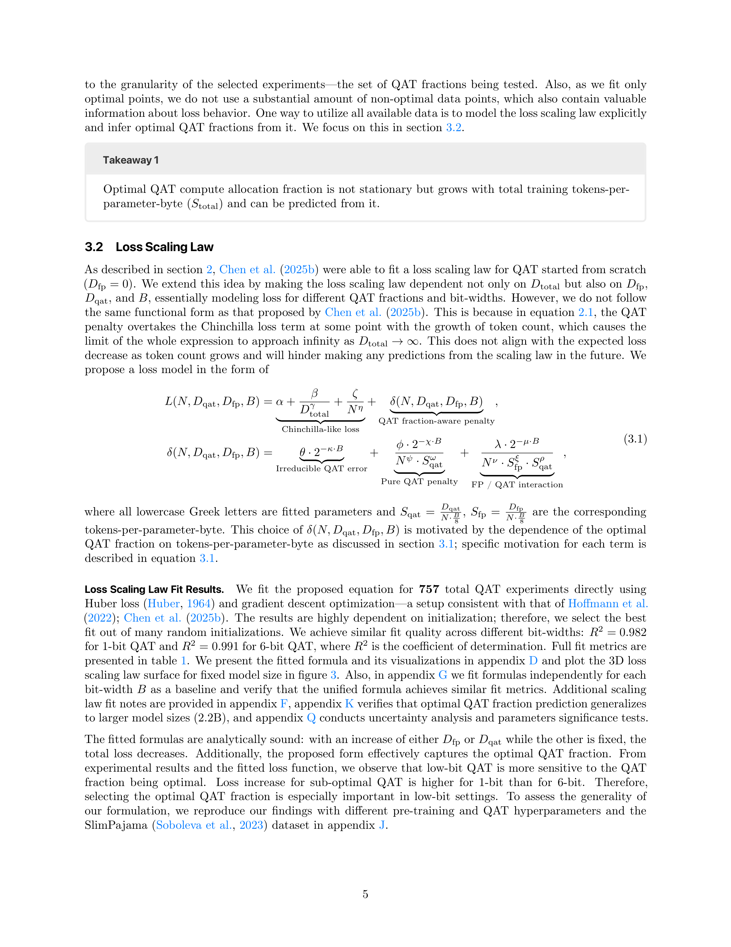
L
(
N, D
qat
, D
fp
, B
) =
α
+
β
D
γ
total
+
ζ
N
η
|
{z
}
Chinchilla-like
loss
+
δ
(
N, D
qat
, D
fp
, B
)
|
{z
}
QAT
fraction-aware
penalty
,
δ
(
N, D
qat
, D
fp
, B
) =
θ
·
2
−
κ
·
B
|
{z
}
Irreducible
QAT
error
+
ϕ
·
2
−
χ
·
B
N
ψ
·
S
ω
qat
|
{z
}
Pure
QAT
penalty
+
λ
·
2
−
µ
·
B
N
ν
·
S
ξ
fp
·
S
ρ
qat
|
{z
}
FP
/
QAT
interaction
,
(3.1)
where
all
lowercase
Greek
letters
are
fitted
parameters
and
S
qat
=
D
qat
N
·
B
8
,
S
fp
=
D
fp
N
·
B
8
are
the
corresponding
tokens-per-parameter-byte.
This
choice
of
δ
(
N, D
qat
, D
fp
, B
)
is
motivated
by
the
dependence
of
the
optimal
QAT
fraction
on
tokens-per-parameter-byte
as
discussed
in
section
3.1
;
specific
motivation
for
each
term
is
described
in
equation
3.1
.
Loss Scaling Law Fit Results.
We
fit
the
proposed
equation
for
757
total
QAT
experiments
directly
using
Huber
loss
(
Huber
,
1964
)
and
gradient
descent
optimization—a
setup
consistent
with
that
of
Hoffmann
et
al.
(
2022
);
Chen
et
al.
(
2025b
).
The
results
are
highly
dependent
on
initialization;
therefore,
we
select
the
best
fit
out
of
many
random
initializations.
We
achieve
similar
fit
quality
across
different
bit-widths:
R
2
= 0
.
982
for 1-bit QAT and
R
2
= 0
.
991
for 6-bit QAT, where
R
2
is the coefficient of determination.
Full fit metrics are
presented
in
table
1
.
We
present
the
fitted
formula
and
its
visualizations
in
appendix
D
and
plot
the
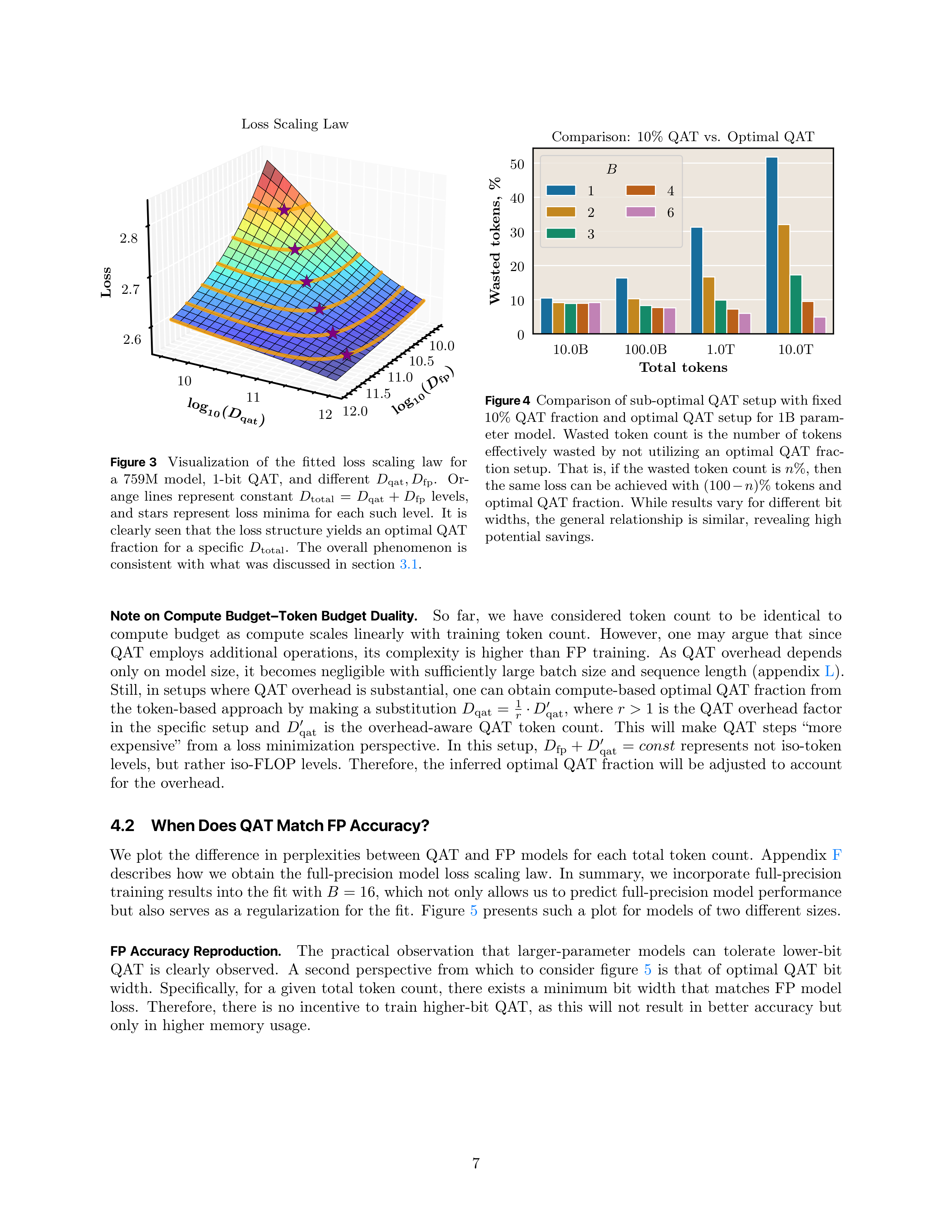
3D
loss
scaling law surface for fixed model size in figure
3
.
Also, in appendix
G
we fit formulas independently for each
bit-width
B
as
a
baseline
and
verify
that
the
unified
formula
achieves
similar
fit
metrics.
Additional
scaling
law fit notes are provided in appendix
F
, appendix
K
verifies that optimal QAT fraction prediction generalizes
to larger model sizes (2.2B), and appendix
Q
conducts uncertainty analysis and parameters significance tests.
The fitted formulas are analytically sound:
with an increase of either
D
fp
or
D
qat
while the other is fixed, the
total
loss
decreases.
Additionally,
the
proposed
form
effectively
captures
the
optimal
QAT
fraction.
From
experimental
results
and
the
fitted
loss
function,
we
observe
that
low-bit
QAT
is
more
sensitive
to
the
QAT
fraction
being
optimal.
Loss
increase
for
sub-optimal
QAT
is
higher
for
1-bit
than
for
6-bit.
Therefore,
selecting
the
optimal
QAT
fraction
is
especially
important
in
low-bit
settings.
To
assess
the
generality
of
our
formulation,
we
reproduce
our
findings
with
different
pre-training
and
QAT
hyperparameters
and
the
SlimPajama
(
Soboleva
et
al.
,
2023
)
dataset
in
appendix
J
.
5
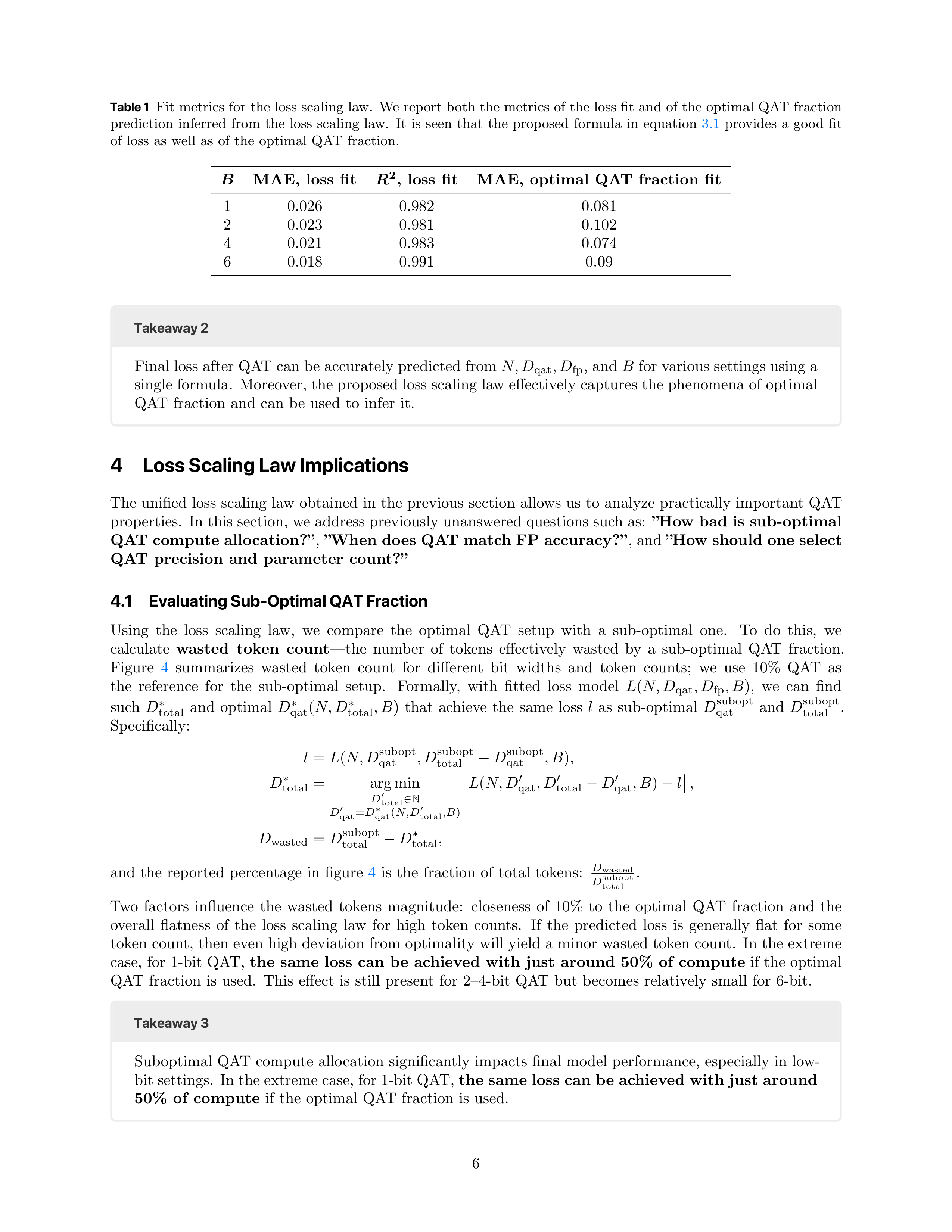
Table 1
Fit
metrics
for
the
loss
scaling
law.
We
report
both
the
metrics
of
the
loss
fit
and
of
the
optimal
QAT
fraction
prediction
inferred
from
the
loss
scaling
law.
It
is
seen
that
the
proposed
formula
in
equation
3.1
provides
a
good
fit
of
loss
as
well
as
of
the
optimal
QAT
fraction.
B
MAE,
loss
fit
R
2
,
loss
fit
MAE,
optimal
QAT
fraction
fit
1
0.026
0.982
0.081
2
0.023
0.981
0.102
4
0.021
0.983
0.074
6
0.018
0.991
0.09
Takeaway 2
Final loss after QAT can be accurately predicted from
N, D
qat
, D
fp
, and
B
for various settings using a
single formula.
Moreover, the proposed loss scaling law effectively captures the phenomena of optimal
QAT
fraction
and
can
be
used
to
infer
it.
4
Loss Scaling Law Implications
The
unified
loss
scaling
law
obtained
in
the
previous
section
allows
us
to
analyze
practically
important
QAT
properties.
In this section, we address previously unanswered questions such as:
”How
bad
is
sub-optimal
QAT
compute
allocation?”
,
”When
does
QAT
match
FP
accuracy?”
, and
”How
should
one
select
QAT
precision
and
parameter
count?”
4.1
Evaluating Sub-Optimal QAT Fraction
Using
the
loss
scaling
law,
we
compare
the
optimal
QAT
setup
with
a
sub-optimal
one.
To
do
this,
we
calculate
wasted
token
count
—the
number
of
tokens
effectively
wasted
by
a
sub-optimal
QAT
fraction.
Figure
4
summarizes
wasted
token
count
for
different
bit
widths
and
token
counts;
we
use
10%
QAT
as
the
reference
for
the
sub-optimal
setup.
Formally,
with
fitted
loss
model
L
(
N, D
qat
, D
fp
, B
)
,
we
can
find
such
D
∗
total
and
optimal
D
∗
qat
(
N, D
∗
total
, B
)
that
achieve
the
same
loss
l
as
sub-optimal
D
subopt
qat
and
D
subopt
total
.
Specifically:
l
=
L
(
N, D
subopt
qat
, D
subopt
total
−
D
subopt
qat
, B
)
,
D
∗
total
=
arg min
D
′
total
∈
N
D
′
qat
=
D
∗
qat
(
N,D
′
total
,B
)
L
(
N, D
′
qat
, D
′
total
−
D
′
qat
, B
)
−
l
,
D
wasted
=
D
subopt
total
−
D
∗
total
,
and
the
reported
percentage
in
figure
4
is
the
fraction
of
total
tokens:
D
wasted
D
subopt
total
.
Two
factors
influence
the
wasted
tokens
magnitude:
closeness
of
10%
to
the
optimal
QAT
fraction
and
the
overall
flatness
of
the
loss
scaling
law
for
high
token
counts.
If
the
predicted
loss
is
generally
flat
for
some
token
count,
then
even
high
deviation
from
optimality
will
yield
a
minor
wasted
token
count.
In
the
extreme
case,
for
1-bit
QAT,
the
same
loss
can
be
achieved
with
just
around
50%
of
compute
if
the
optimal
QAT
fraction
is
used.
This
effect
is
still
present
for
2–4-bit
QAT
but
becomes
relatively
small
for
6-bit.
Takeaway 3
Suboptimal
QAT
compute
allocation
significantly
impacts
final
model
performance,
especially
in
low-
bit settings.
In the extreme case, for 1-bit QAT,
the
same
loss
can
be
achieved
with
just
around
50%
of
compute
if
the
optimal
QAT
fraction
is
used.
6
10
.
0
10
.
5
11
.
0
11
.
5
12
.
0
log
10
(
D
fp
)
10
11
12
log
10
(
D
qat
)
2
.
6
2
.
7
2
.
8
Loss
Loss
Scaling
Law
Figure 3
Visualization
of
the
fitted
loss
scaling
law
for
a
759M
model,
1-bit
QAT,
and
different
D
qat
, D
fp
.
Or-
ange
lines
represent
constant
D
total
=
D
qat
+
D
fp
levels,
and
stars
represent
loss
minima
for
each
such
level.
It
is
clearly seen that the loss structure yields an optimal QAT
fraction
for
a
specific
D
total
.
The
overall
phenomenon
is
consistent
with
what
was
discussed
in
section
3.1
.
10.0B
100.0B
1.0T
10.0T
Total
tokens
0
10
20
30
40
50
Wasted
tokens,
%
Comparison:
10%
QAT
vs.
Optimal
QAT
B
1
2
3
4
6
Figure 4
Comparison of sub-optimal QAT setup with fixed
10%
QAT
fraction
and
optimal
QAT
setup
for
1B
param-
eter
model.
Wasted
token
count
is
the
number
of
tokens
effectively
wasted
by
not
utilizing
an
optimal
QAT
frac-
tion setup.
That is,
if the wasted token count is
n
%
,
then
the same loss can be achieved with
(100
−
n
)%
tokens and
optimal QAT fraction.
While results vary for different bit
widths,
the
general
relationship
is
similar,
revealing
high
potential
savings.
Note on Compute Budget–Token Budget Duality.
So
far,
we
have
considered
token
count
to
be
identical
to
compute
budget
as
compute
scales
linearly
with
training
token
count.
However,
one
may
argue
that
since
QAT
employs
additional
operations,
its
complexity
is
higher
than
FP
training.
As
QAT
overhead
depends
only
on
model
size,
it
becomes
negligible
with
sufficiently
large
batch
size
and
sequence
length
(appendix
L
).
Still, in setups where QAT overhead is substantial, one can obtain compute-based optimal QAT fraction from
the
token-based
approach
by
making
a
substitution
D
qat
=
1
r
·
D
′
qat
,
where
r
>
1
is
the
QAT
overhead
factor
in
the
specific
setup
and
D
′
qat
is
the
overhead-aware
QAT
token
count.
This
will
make
QAT
steps
“more
expensive”
from
a
loss
minimization
perspective.
In
this
setup,
D
fp
+
D
′
qat
=
const
represents
not
iso-token
levels,
but
rather
iso-FLOP
levels.
Therefore,
the
inferred
optimal
QAT
fraction
will
be
adjusted
to
account
for
the
overhead.
4.2
When Does QAT Match FP Accuracy
?
We
plot
the
difference
in
perplexities
between
QAT
and
FP
models
for
each
total
token
count.
Appendix
F
describes
how
we
obtain
the
full-precision
model
loss
scaling
law.
In
summary,
we
incorporate
full-precision
training results into the fit with
B
= 16
, which not only allows us to predict full-precision model performance
but
also
serves
as
a
regularization
for
the
fit.
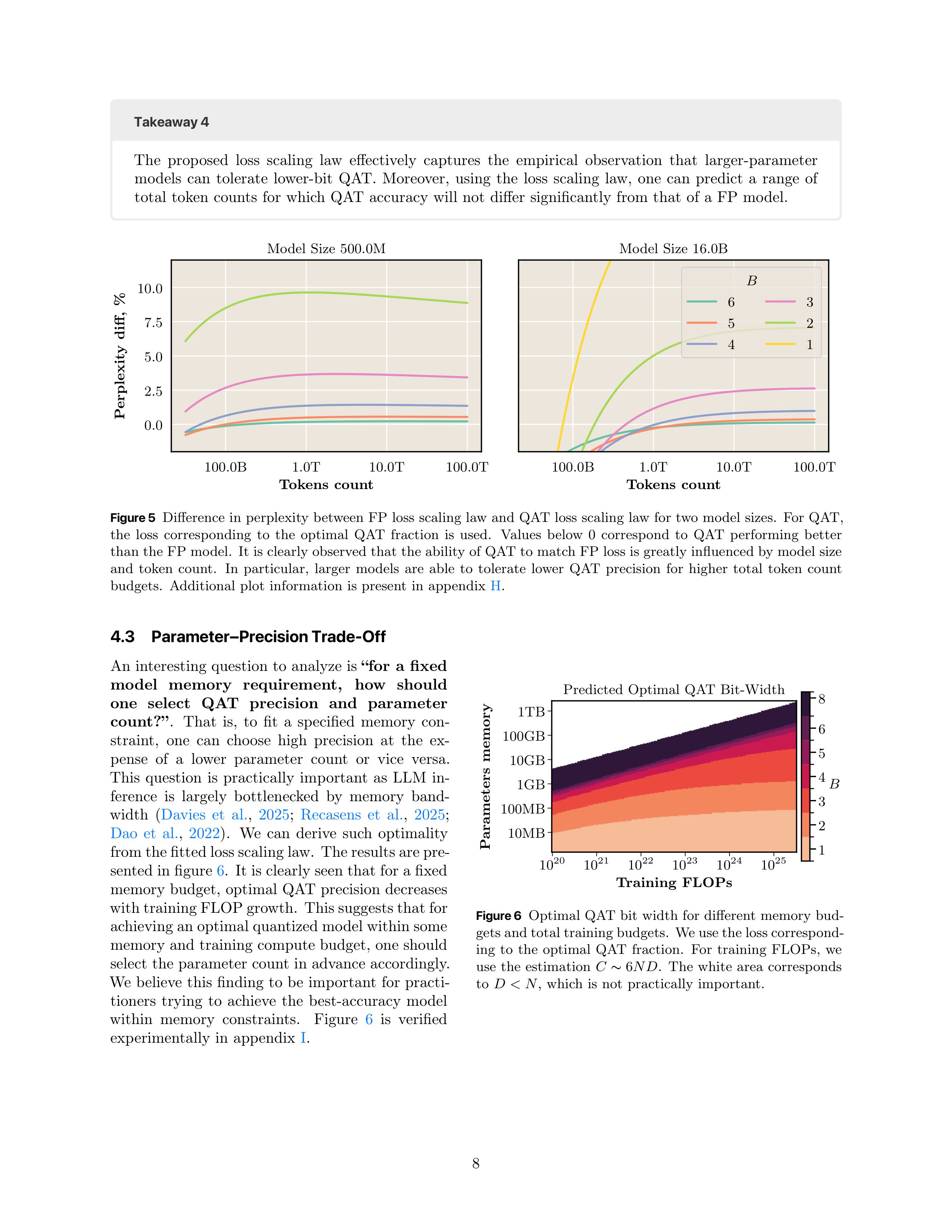
Figure
5
presents
such
a
plot
for
models
of
two
different
sizes.
FP Accuracy Reproduction.
The
practical
observation
that
larger-parameter
models
can
tolerate
lower-bit
QAT
is
clearly
observed.
A
second
perspective
from
which
to
consider
figure
5
is
that
of
optimal
QAT
bit
width.
Specifically,
for
a
given
total
token
count,
there
exists
a
minimum
bit
width
that
matches
FP
model
loss.
Therefore,
there
is
no
incentive
to
train
higher-bit
QAT,
as
this
will
not
result
in
better
accuracy
but
only
in
higher
memory
usage.
7

Takeaway 4
The
proposed
loss
scaling
law
effectively
captures
the
empirical
observation
that
larger-parameter
models
can
tolerate
lower-bit
QAT.
Moreover,
using
the
loss
scaling
law,
one
can
predict
a
range
of
total
token
counts
for
which
QAT
accuracy
will
not
differ
significantly
from
that
of
a
FP
model.
100.0B
1.0T
10.0T
100.0T
Tokens
count
0
.
0
2
.
5
5
.
0
7
.
5
10
.
0
Perplexity
diff,
%
Model
Size
500.0M
100.0B
1.0T
10.0T
100.0T
Tokens
count
Model
Size
16.0B
B
6
5
4
3
2
1
Figure 5
Difference
in
perplexity
between
FP
loss
scaling
law
and
QAT
loss
scaling
law
for
two
model
sizes.
For
QAT,
the
loss
corresponding
to
the
optimal
QAT
fraction
is
used.
Values
below
0
correspond
to
QAT
performing
better
than the FP model.
It is clearly observed that the ability of QAT to match FP loss is greatly influenced by model size
and
token
count.
In
particular,
larger
models
are
able
to
tolerate
lower
QAT
precision
for
higher
total
token
count
budgets.
Additional
plot
information
is
present
in
appendix
H
.
4.3
Parameter–Precision Trade-Off
10
20
10
21
10
22
10
23
10
24
10
25
Training
FLOPs
10MB
100MB
1GB
10GB
100GB
1TB
Parameters
memory
Predicted
Optimal
QAT
Bit-Width
1
2
3
4
5
6
8
B
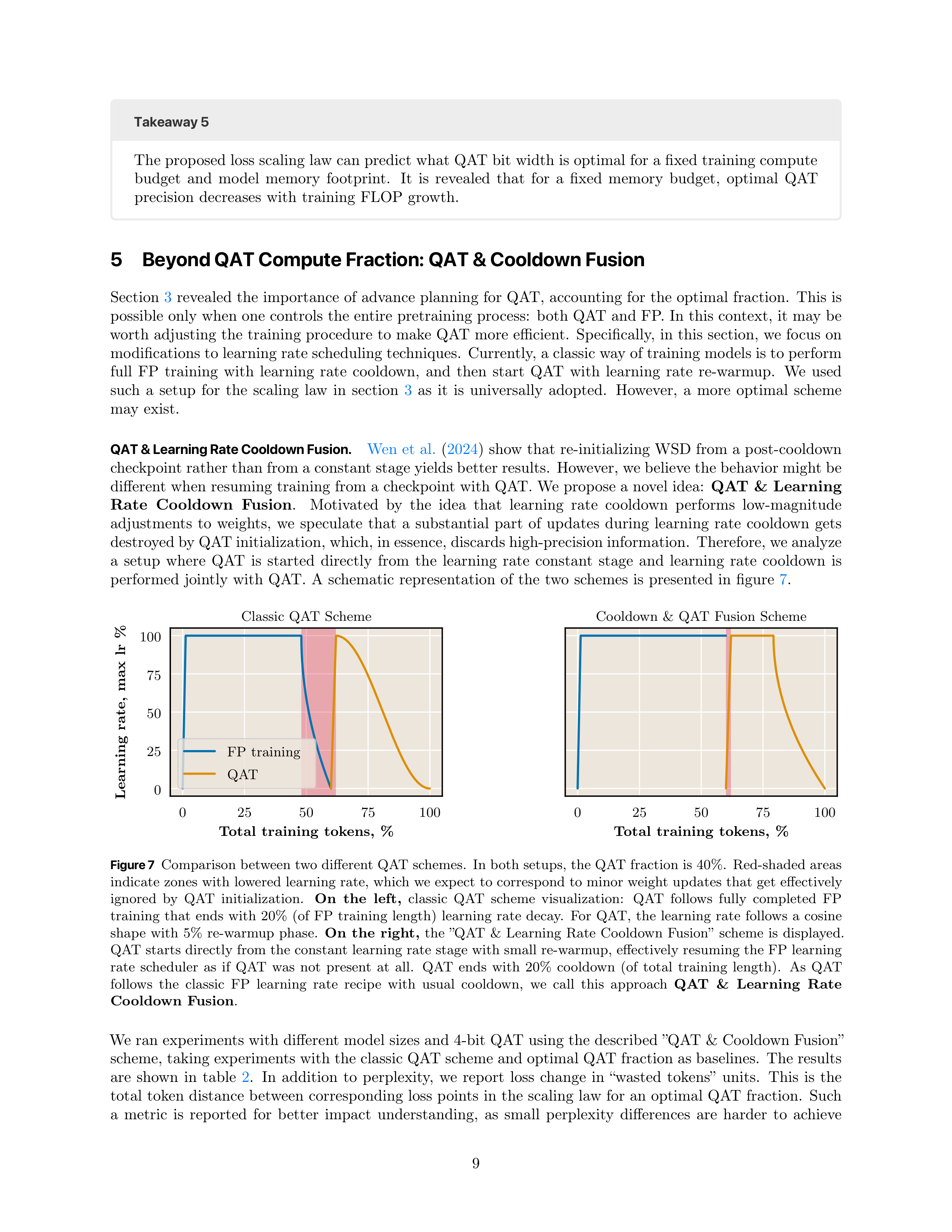
Figure 6
Optimal
QAT
bit
width
for
different
memory
bud-
gets and total training budgets.
We use the loss correspond-
ing
to
the
optimal
QAT
fraction.
For
training
FLOPs,
we
use
the
estimation
C
∼
6
ND
.
The
white
area
corresponds
to
D
< N
,
which
is
not
practically
important.
An
interesting
question
to
analyze
is
“for
a
fixed
model
memory
requirement,
how
should
one
select
QAT
precision
and
parameter
count?”
.
That
is,
to
fit
a
specified
memory
con-
straint,
one
can
choose
high
precision
at
the
ex-
pense
of
a
lower
parameter
count
or
vice
versa.
This
question
is
practically
important
as
LLM
in-
ference
is
largely
bottlenecked
by
memory
band-
width
(
Davies
et
al.
,
2025
;
Recasens
et
al.
,
2025
;
Dao
et
al.
,
2022
).
We
can
derive
such
optimality
from the fitted loss scaling law.
The results are pre-
sented in figure
6
.
It is clearly seen that for a fixed
memory
budget,
optimal
QAT
precision
decreases
with training FLOP growth.
This suggests that for
achieving an optimal quantized model within some
memory
and
training
compute
budget,
one
should
select
the
parameter
count
in
advance
accordingly.
We
believe
this
finding
to
be
important
for
practi-
tioners
trying
to
achieve
the
best-accuracy
model
within
memory
constraints.
Figure
6
is
verified
experimentally
in
appendix
I
.
8
Takeaway 5
The proposed loss scaling law can predict what QAT bit width is optimal for a fixed training compute
budget
and
model
memory
footprint.
It
is
revealed
that
for
a
fixed
memory
budget,
optimal
QAT
precision
decreases
with
training
FLOP
growth.
5
Beyond QAT Compute Fraction: QAT & Cooldown Fusion
Section
3
revealed
the
importance
of
advance
planning
for
QAT,
accounting
for
the
optimal
fraction.
This
is
possible
only
when
one
controls
the
entire
pretraining
process:
both
QAT
and
FP.
In
this
context,
it
may
be
worth
adjusting
the
training
procedure
to
make
QAT
more
efficient.
Specifically,
in
this
section,
we
focus
on
modifications to learning rate scheduling techniques.
Currently, a classic way of training models is to perform
full
FP
training
with
learning
rate
cooldown,
and
then
start
QAT
with
learning
rate
re-warmup.
We
used
such
a
setup
for
the
scaling
law
in
section
3
as
it
is
universally
adopted.
However,
a
more
optimal
scheme
may
exist.
QAT & Learning Rate Cooldown Fusion.
Wen
et
al.
(
2024
)
show
that
re-initializing
WSD
from
a
post-cooldown
checkpoint rather than from a constant stage yields better results.
However, we believe the behavior might be
different
when
resuming
training
from
a
checkpoint
with
QAT.
We
propose
a
novel
idea:
QAT
&
Learning
Rate
Cooldown
Fusion
.
Motivated
by
the
idea
that
learning
rate
cooldown
performs
low-magnitude
adjustments
to
weights,
we
speculate
that
a
substantial
part
of
updates
during
learning
rate
cooldown
gets
destroyed by QAT initialization, which, in essence, discards high-precision information.
Therefore, we analyze
a
setup
where
QAT
is
started
directly
from
the
learning
rate
constant
stage
and
learning
rate
cooldown
is
performed
jointly
with
QAT.
A
schematic
representation
of
the
two
schemes
is
presented
in
figure
7
.
0
25
50
75
100
Total
training
tokens,
%
0
25
50
75
100
Learning
rate,
max
lr
%
Classic
QAT
Scheme
FP
training
QAT
0
25
50
75
100
Total
training
tokens,
%
Cooldown
&
QAT
Fusion
Scheme
Figure 7
Comparison
between
two
different
QAT
schemes.
In both
setups,
the QAT fraction
is 40%.
Red-shaded
areas
indicate
zones
with
lowered
learning
rate,
which
we
expect
to
correspond
to
minor
weight
updates
that
get
effectively
ignored
by
QAT
initialization.
On
the
left,
classic
QAT
scheme
visualization:
QAT
follows
fully
completed
FP
training
that
ends
with
20%
(of
FP
training
length)
learning
rate
decay.
For
QAT,
the
learning
rate
follows
a
cosine
shape
with
5%
re-warmup
phase.
On
the
right,
the
”QAT
&
Learning
Rate
Cooldown
Fusion”
scheme
is
displayed.
QAT
starts
directly
from
the
constant
learning
rate
stage
with
small
re-warmup,
effectively
resuming
the
FP
learning
rate
scheduler
as
if
QAT
was
not
present
at
all.
QAT
ends
with
20%
cooldown
(of
total
training
length).
As
QAT
follows
the
classic
FP
learning
rate
recipe
with
usual
cooldown,
we
call
this
approach
QAT
&
Learning
Rate
Cooldown
Fusion
.
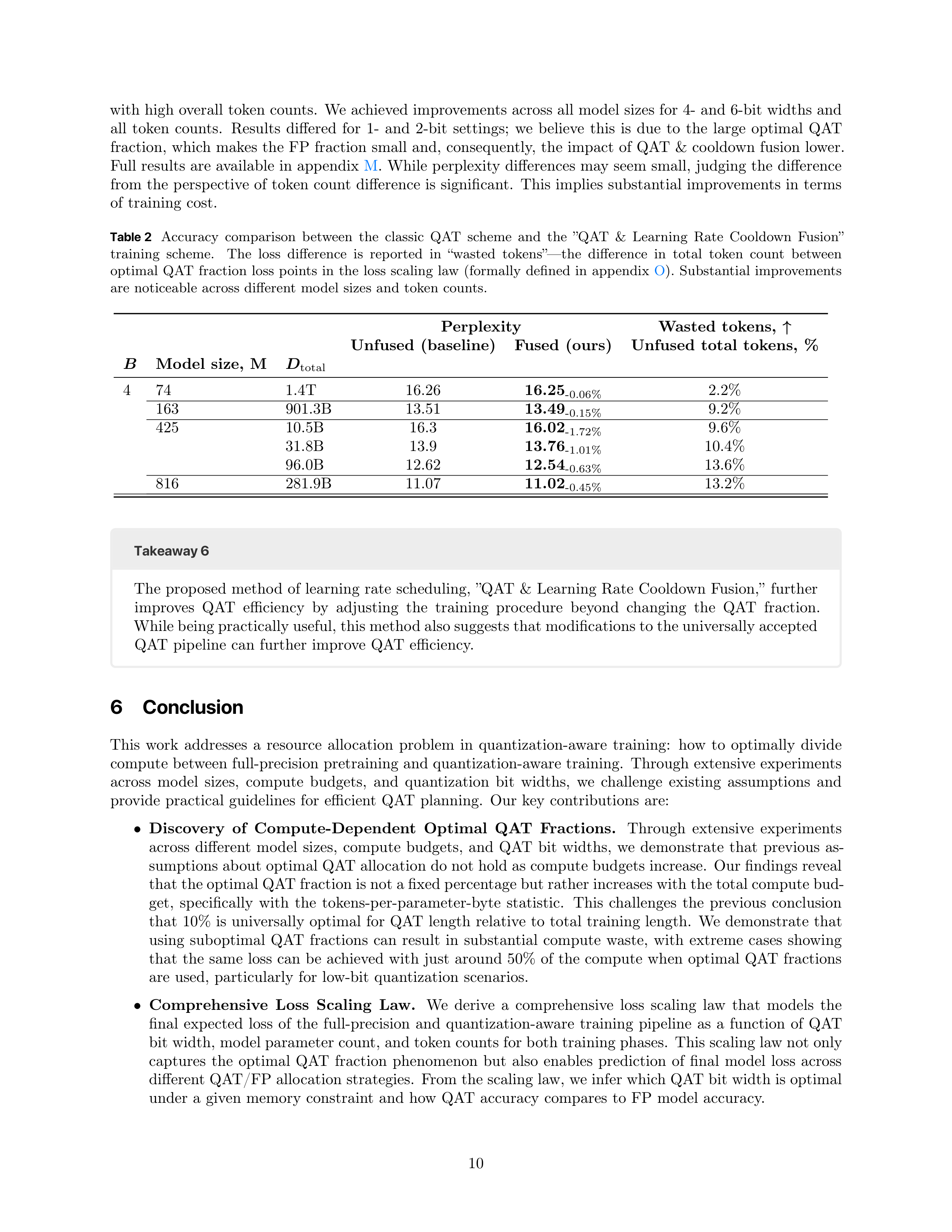
We ran experiments with different model sizes and 4-bit QAT using the described ”QAT & Cooldown Fusion”
scheme, taking experiments with the classic QAT scheme and optimal QAT fraction as baselines.
The results
are
shown
in
table
2
.
In
addition
to
perplexity,
we
report
loss
change
in
“wasted
tokens”
units.
This
is
the
total
token
distance
between
corresponding
loss
points
in
the
scaling
law
for
an
optimal
QAT
fraction.
Such
a
metric
is
reported
for
better
impact
understanding,
as
small
perplexity
differences
are
harder
to
achieve
9
with
high
overall
token
counts.
We
achieved
improvements
across
all
model
sizes
for
4-
and
6-bit
widths
and
all
token
counts.
Results
differed
for
1-
and
2-bit
settings;
we
believe
this
is
due
to
the
large
optimal
QAT
fraction,
which
makes
the
FP
fraction
small
and,
consequently,
the
impact
of
QAT
&
cooldown
fusion
lower.
Full
results
are
available
in
appendix
M
.
While
perplexity
differences
may
seem
small,
judging
the
difference
from
the
perspective
of
token
count
difference
is
significant.
This
implies
substantial
improvements
in
terms
of
training
cost.
Table 2
Accuracy
comparison
between
the
classic
QAT
scheme
and
the
”QAT
&
Learning
Rate
Cooldown
Fusion”
training
scheme.
The
loss
difference
is
reported
in
“wasted
tokens”—the
difference
in
total
token
count
between
optimal
QAT
fraction
loss
points
in
the
loss
scaling
law
(formally
defined
in
appendix
O
).
Substantial
improvements
are
noticeable
across
different
model
sizes
and
token
counts.
Perplexity
Wasted
tokens,
↑
Unfused
(baseline)
Fused
(ours)
Unfused
total
tokens,
%
B
Model
size,
M
D
total
4
74
1.4T
16.26
16.25
-0.06%
2.2%
163
901.3B
13.51
13.49
-0.15%
9.2%
425
10.5B
16.3
16.02
-1.72%
9.6%
31.8B
13.9
13.76
-1.01%
10.4%
96.0B
12.62
12.54
-0.63%
13.6%
816
281.9B
11.07
11.02
-0.45%
13.2%
Takeaway 6
The
proposed
method
of
learning
rate
scheduling,
”QAT
&
Learning
Rate
Cooldown
Fusion,”
further
improves
QAT
efficiency
by
adjusting
the
training
procedure
beyond
changing
the
QAT
fraction.
While being practically useful, this method also suggests that modifications to the universally accepted
QAT
pipeline
can
further
improve
QAT
efficiency.
6
Conclusion
This
work
addresses
a
resource
allocation
problem
in
quantization-aware
training:
how
to
optimally
divide
compute
between
full-precision
pretraining
and
quantization-aware
training.
Through
extensive
experiments
across
model
sizes,
compute
budgets,
and
quantization
bit
widths,
we
challenge
existing
assumptions
and
provide
practical
guidelines
for
efficient
QAT
planning.
Our
key
contributions
are:
•
Discovery
of
Compute-Dependent
Optimal
QAT
Fractions.
Through
extensive
experiments
across
different
model
sizes,
compute
budgets,
and
QAT
bit
widths,
we
demonstrate
that
previous
as-
sumptions about optimal QAT allocation do not hold as compute budgets increase.
Our findings reveal
that the optimal QAT fraction is not a fixed percentage but rather increases with the total compute bud-
get,
specifically
with
the
tokens-per-parameter-byte
statistic.
This
challenges
the
previous
conclusion
that
10%
is
universally
optimal
for
QAT
length
relative
to
total
training
length.
We
demonstrate
that
using
suboptimal
QAT
fractions
can
result
in
substantial
compute
waste,
with
extreme
cases
showing
that
the
same
loss
can
be
achieved
with
just
around
50%
of
the
compute
when
optimal
QAT
fractions
are
used,
particularly
for
low-bit
quantization
scenarios.
•
Comprehensive
Loss
Scaling
Law.
We
derive
a
comprehensive
loss
scaling
law
that
models
the
final
expected
loss
of
the
full-precision
and
quantization-aware
training
pipeline
as
a
function
of
QAT
bit width, model parameter count, and token counts for both training phases.
This scaling law not only
captures
the
optimal
QAT
fraction
phenomenon
but
also
enables
prediction
of
final
model
loss
across
different QAT/FP allocation strategies.
From the scaling law, we infer which QAT bit width is optimal
under
a
given
memory
constraint
and
how
QAT
accuracy
compares
to
FP
model
accuracy.
10
•
Cooldown
and
QAT
Fusion
Technique.
We
introduce
a
novel
approach
that
performs
learning
rate
decay
jointly
with
quantization-aware
training,
eliminating
redundant
full-precision
updates
and
achieving
significant
compute
savings.
While
being
practically
useful,
this
method
also
suggests
that
modifications
to
the
universally
accepted
QAT
pipeline
can
further
improve
QAT
efficiency.
Limitations.
While
we
checked
the
generality
of
our
formulation
by
performing
experiments
with
a
different
dataset
and
hyperparameters
in
appendix
J
,
our
work
still
focuses
on
a
specific
LLM
architecture,
and
exact
results
may
differ
for
different
model
types.
However,
we
expect
the
overall
observed
phenomena
to
be
consistent
across
different
architectures
and
datasets.
Future Work.
We
identify
several
research
directions
worth
exploring.
First,
the
relationship
between
the
optimal
QAT
fraction
and
pretraining
precision
remains
unknown.
This
direction
is
especially
interesting
with
the
emergence
of
8-bit
floating-point
training
(
Peng
et
al.
,
2023
)
and
even
4-bit
training
(
Zhou
et
al.
,
2025b
;
Wang
et
al.
,
2025
).
Second,
we
are
interested
in
how
the
observed
phenomena
are
preserved
across
different
training
stages.
Specifically,
how
does
the
optimal
QAT
fraction
change
when
the
full-precision
training
stage
incorporates
additional
stages
such
as
Supervised
Fine-Tuning
(SFT)
(
Ouyang
et
al.
,
2022
),
Reinforcement
Learning
(RL)
(
Rafailov
et
al.
,
2023
;
Schulman
et
al.
,
2017
),
or
multimodal
training?
We
speculate
on
these
questions
in
appendix
R
.
Reproducibility Statement.
We
report
exact
hyperparameters
and
training
approaches
used
in
appendix
A
.
Additional
experimental
information
that
should
facilitate
reproduction
is
summarized
in
appendix
B
,
C
,
and
N
.
Ethics Statement:
LLM Use Disclosure.
LLMs
such
as
Anthropic
(
2025
);
Mistral
AI
(
2025
)
were
used
in
the
preparation
of
this
paper
exclusively
for
improving
grammar
and
wording.
References
Loubna Ben Allal, Anton Lozhkov, Elie Bakouch, Gabriel Martín Blázquez, Guilherme Penedo, Lewis Tunstall, Andrés
Marafioti,
Hynek
Kydlícek,
Agustín
Piqueres
Lajarín,
Vaibhav
Srivastav,
Joshua
Lochner,
Caleb
Fahlgren,
Xuan-
Son
Nguyen,
Clémentine
Fourrier,
Ben
Burtenshaw,
Hugo
Larcher,
Haojun
Zhao,
Cyril
Zakka,
Mathieu
Morlon,
Colin
Raffel,
Leandro
von
Werra,
and
Thomas
Wolf.
Smollm2:
When
smol
goes
big
-
data-centric
training
of
a
small language model.
CoRR
, abs/2502.02737,
2025.
doi:
10.48550/ARXIV.2502.02737.
URL
https://doi.org/10.48550/
arXiv.2502.02737
.
Anthropic.
Claude
[large
language
model],
2025.
URL
https://www.anthropic.com
.
Project
Apertus,
Alejandro
Hernández-Cano,
Alexander
Hägele,
Allen
Hao
Huang,
Angelika
Romanou,
Antoni-Joan
Solergibert,
Barna
Pasztor,
Bettina
Messmer,
Dhia
Garbaya,
Eduard
Frank
Ďurech,
Ido
Hakimi,
Juan
García
Giraldo, Mete Ismayilzada, Negar Foroutan, Skander Moalla, Tiancheng Chen, Vinko Sabolčec, Yixuan Xu, Michael
Aerni, Badr AlKhamissi, Inés Altemir Mariñas, Mohammad Hossein Amani, Matin Ansaripour, Ilia Badanin, Harold
Benoit,
Emanuela
Boros,
Nicholas
Browning,
Fabian
Bösch,
Maximilian
Böther,
Niklas
Canova,
Camille
Challier,
Clement Charmillot, Jonathan Coles, Jan Deriu, Arnout Devos, Lukas Drescher, Daniil Dzenhaliou, Maud Ehrmann,
Dongyang Fan, Simin Fan, Silin Gao, Miguel Gila, María Grandury, Diba Hashemi, Alexander Hoyle, Jiaming Jiang,
Mark
Klein,
Andrei
Kucharavy,
Anastasiia
Kucherenko,
Frederike
Lübeck,
Roman
Machacek,
Theofilos
Manitaras,
Andreas Marfurt, Kyle Matoba, Simon Matrenok, Henrique Mendonça, Fawzi Roberto Mohamed, Syrielle Montariol,
Luca
Mouchel,
Sven
Najem-Meyer,
Jingwei
Ni,
Gennaro
Oliva,
Matteo
Pagliardini,
Elia
Palme,
Andrei
Panferov,
Léo
Paoletti,
Marco
Passerini,
Ivan
Pavlov,
Auguste
Poiroux,
Kaustubh
Ponkshe,
Nathan
Ranchin,
Javi
Rando,
Mathieu
Sauser,
Jakhongir
Saydaliev,
Muhammad
Ali
Sayfiddinov,
Marian
Schneider,
Stefano
Schuppli,
Marco
Scialanga, Andrei Semenov, Kumar Shridhar, Raghav Singhal, Anna Sotnikova, Alexander Sternfeld, Ayush Kumar
Tarun,
Paul
Teiletche,
Jannis
Vamvas,
Xiaozhe
Yao,
Hao
Zhao,
Alexander
Ilic,
Ana
Klimovic,
Andreas
Krause,
Caglar Gulcehre, David Rosenthal, Elliott Ash, Florian Tramèr, Joost VandeVondele, Livio Veraldi, Martin Rajman,
Thomas
Schulthess,
Torsten
Hoefler,
Antoine
Bosselut,
Martin
Jaggi,
and
Imanol
Schlag.
Apertus:
Democratizing
open
and
compliant
llms
for
global
language
environments,
2025.
URL
https://arxiv.org/abs/2509.14233
.
Ron
Banner,
Yury
Nahshan,
and
Daniel
Soudry.
Post
training
4-bit
quantization
of
convolutional
networks
for
rapid-deployment.
In
Hanna
M.
Wallach,
Hugo
Larochelle,
Alina
Beygelzimer,
Florence
d’Alché-Buc,
Emily
B.
11
Fox,
and
Roman
Garnett
(eds.),
Advances
in
Neural
Information
Processing
Systems
32:
Annual
Conference
on
Neural
Information
Processing
Systems
2019,
NeurIPS
2019,
December
8-14,
2019,
Vancouver,
BC,
Canada
,
pp.
7948–7956,
2019.
URL
https://proceedings.neurips.cc/paper/2019/hash/c0a62e133894cdce435bcb4a5df1db2d-Abstract.html
.
Yoshua
Bengio,
Nicholas
Léonard,
and
Aaron
C.
Courville.
Estimating
or
propagating
gradients
through
stochastic
neurons
for
conditional
computation.
CoRR
,
abs/1308.3432,
2013.
URL
http://arxiv.org/abs/1308.3432
.
Xiao
Bi,
Deli
Chen,
Guanting
Chen,
Shanhuang
Chen,
Damai
Dai,
Chengqi
Deng,
Honghui
Ding,
Kai
Dong,
Qiushi
Du, Zhe Fu, Huazuo Gao, Kaige Gao, Wenjun Gao, Ruiqi Ge, Kang Guan, Daya Guo, Jianzhong Guo, Guangbo Hao,
Zhewen Hao, Ying He, Wenjie Hu, Panpan Huang, Erhang Li, Guowei Li, Jiashi Li, Yao Li, Y. K. Li, Wenfeng Liang,
Fangyun
Lin,
Alex
X.
Liu,
Bo
Liu,
Wen
Liu,
Xiaodong
Liu,
Xin
Liu,
Yiyuan
Liu,
Haoyu
Lu,
Shanghao
Lu,
Fuli
Luo,
Shirong
Ma,
Xiaotao
Nie,
Tian
Pei,
Yishi
Piao,
Junjie
Qiu,
Hui
Qu,
Tongzheng
Ren,
Zehui
Ren,
Chong
Ruan,
Zhangli
Sha,
Zhihong
Shao,
Junxiao
Song,
Xuecheng
Su,
Jingxiang
Sun,
Yaofeng
Sun,
Minghui
Tang,
Bingxuan
Wang,
Peiyi
Wang,
Shiyu
Wang,
Yaohui
Wang,
Yongji
Wang,
Tong
Wu,
Y.
Wu,
Xin
Xie,
Zhenda
Xie,
Ziwei
Xie,
Yiliang Xiong,
Hanwei Xu,
R. X. Xu,
Yanhong Xu,
Dejian Yang,
Yuxiang You,
Shuiping Yu,
Xingkai Yu,
B. Zhang,
Haowei
Zhang,
Lecong
Zhang,
Liyue
Zhang,
Mingchuan
Zhang,
Minghua
Zhang,
Wentao
Zhang,
Yichao
Zhang,
Chenggang
Zhao,
Yao
Zhao,
Shangyan
Zhou,
Shunfeng
Zhou,
Qihao
Zhu,
and
Yuheng
Zou.
Deepseek
LLM:
scaling
open-source
language
models
with
longtermism.
CoRR
,
abs/2401.02954,
2024.
doi:
10.48550/ARXIV.2401.02954.
URL
https://doi.org/10.48550/arXiv.2401.02954
.
Mengzhao Chen, Wenqi Shao, Peng Xu, Jiahao Wang, Peng Gao, Kaipeng Zhang, and Ping Luo.
Efficientqat:
Efficient
quantization-aware
training
for
large
language
models.
In
Wanxiang
Che,
Joyce
Nabende,
Ekaterina
Shutova,
and
Mohammad
Taher
Pilehvar
(eds.),
Proceedings
of
the
63rd
Annual
Meeting
of
the
Association
for
Computational
Linguistics
(Volume
1:
Long
Papers),
ACL
2025,
Vienna,
Austria,
July
27
-
August
1,
2025
,
pp.
10081–10100.
Association
for
Computational
Linguistics,
2025a.
URL
https://aclanthology.org/2025.acl-long.498/
.
Mengzhao
Chen,
Chaoyi
Zhang,
Jing
Liu,
Yutao
Zeng,
Zeyue
Xue,
Zhiheng
Liu,
Yunshui
Li,
Jin
Ma,
Jie
Huang,
Xun
Zhou,
and
Ping
Luo.
Scaling
law
for
quantization-aware
training.
CoRR
,
abs/2505.14302,
2025b.
doi:
10.48550/
ARXIV.2505.14302.
URL
https://doi.org/10.48550/arXiv.2505.14302
.
Tri
Dao,
Daniel
Y.
Fu,
Stefano
Ermon,
Atri
Rudra,
and
Christopher
Ré.
Flashattention:
Fast
and
memory-efficient
exact
attention
with
io-awareness.
In
Sanmi
Koyejo,
S.
Mohamed,
A.
Agarwal,
Danielle
Belgrave,
K.
Cho,
and
A.
Oh
(eds.),
Advances
in
Neural
Information
Processing
Systems
35:
Annual
Conference
on
Neural
Information
Processing
Systems
2022,
NeurIPS
2022,
New
Orleans,
LA,
USA,
November
28
-
December
9,
2022
,
2022.
URL
http://papers.nips.cc/paper_files/paper/2022/hash/67d57c32e20fd0a7a302cb81d36e40d5-Abstract-Conference.html
.
Michael
Davies,
Neal
Clayton
Crago,
Karthikeyan
Sankaralingam,
and
Christos
Kozyrakis.
Efficient
LLM
inference:
Bandwidth,
compute,
synchronization,
and
capacity
are
all
you
need.
CoRR
,
abs/2507.14397,
2025.
doi:
10.48550/
ARXIV.2507.14397.
URL
https://doi.org/10.48550/arXiv.2507.14397
.
DeepSeek-AI,
Daya
Guo,
Dejian
Yang,
Haowei
Zhang,
Junxiao
Song,
Ruoyu
Zhang,
Runxin
Xu,
Qihao
Zhu,
Shirong
Ma,
Peiyi
Wang,
Xiao
Bi,
Xiaokang
Zhang,
Xingkai
Yu,
Yu
Wu,
Z.
F.
Wu,
Zhibin
Gou,
Zhihong
Shao,
Zhuoshu
Li,
Ziyi
Gao,
Aixin
Liu,
Bing
Xue,
Bingxuan
Wang,
Bochao
Wu,
Bei
Feng,
Chengda
Lu,
Chenggang
Zhao,
Chengqi
Deng,
Chenyu
Zhang,
Chong
Ruan,
Damai
Dai,
Deli
Chen,
Dongjie
Ji,
Erhang
Li,
Fangyun
Lin,
Fucong
Dai,
Fuli
Luo,
Guangbo
Hao,
Guanting
Chen,
Guowei
Li,
H.
Zhang,
Han
Bao,
Hanwei
Xu,
Haocheng
Wang,
Honghui
Ding,
Huajian
Xin,
Huazuo
Gao,
Hui
Qu,
Hui
Li,
Jianzhong
Guo,
Jiashi
Li,
Jiawei
Wang,
Jingchang
Chen,
Jingyang
Yuan,
Junjie
Qiu,
Junlong
Li,
J.
L.
Cai,
Jiaqi
Ni,
Jian
Liang,
Jin
Chen,
Kai
Dong,
Kai
Hu,
Kaige
Gao,
Kang
Guan,
Kexin
Huang,
Kuai
Yu,
Lean
Wang,
Lecong
Zhang,
Liang
Zhao,
Litong
Wang,
Liyue
Zhang,
Lei
Xu,
Leyi
Xia,
Mingchuan
Zhang,
Minghua
Zhang,
Minghui
Tang,
Meng
Li,
Miaojun
Wang,
Mingming
Li,
Ning
Tian,
Panpan
Huang,
Peng
Zhang,
Qiancheng
Wang,
Qinyu
Chen,
Qiushi
Du,
Ruiqi
Ge,
Ruisong
Zhang,
Ruizhe
Pan,
Runji
Wang,
R.
J.
Chen,
R.
L.
Jin,
Ruyi
Chen,
Shanghao
Lu,
Shangyan
Zhou,
Shanhuang
Chen,
Shengfeng
Ye,
Shiyu
Wang,
Shuiping
Yu,
Shunfeng
Zhou,
Shuting
Pan,
and
S.
S.
Li.
Deepseek-r1:
Incentivizing
reasoning
capability
in
llms
via
reinforcement
learning.
CoRR
,
abs/2501.12948,
2025.
doi:
10.48550/ARXIV.2501.12948.
URL
https://doi.org/10.48550/arXiv.2501.12948
.
Aleksandr
Dremov,
Alexander
Hägele,
Atli
Kosson,
and
Martin
Jaggi.
Training
dynamics
of
the
cooldown
stage
in
warmup-stable-decay
learning
rate
scheduler.
Trans.
Mach.
Learn.
Res.
,
2025,
2025.
URL
https://openreview.net/forum
?
id=ZnSYEcZod3
.
Steven
K.
Esser,
Jeffrey
L.
McKinstry,
Deepika
Bablani,
Rathinakumar
Appuswamy,
and
Dharmendra
S.
Modha.
Learned
step
size
quantization.
In
International
Conference
on
Learning
Representations
,
2020.
URL
https:
//openreview.net/forum
?id=rkgO66VKDS
.
Elias
Frantar,
Saleh
Ashkboos,
Torsten
Hoefler,
and
Dan
Alistarh.
GPTQ:
accurate
post-training
quantization
12
for
generative
pre-trained
transformers.
CoRR
,
abs/2210.17323,
2022.
doi:
10.48550/ARXIV.2210.17323.
URL
https://doi.org/10.48550/arXiv.2210.17323
.
Alexander
Hägele,
Elie
Bakouch,
Atli
Kosson,
Loubna
Ben
Allal,
Leandro
von
Werra,
and
Martin
Jaggi.
Scaling
laws
and
compute-optimal
training
beyond
fixed
training
durations.
In
Amir
Globersons,
Lester
Mackey,
Danielle
Belgrave,
Angela
Fan,
Ulrich
Paquet,
Jakub
M.
Tomczak,
and
Cheng
Zhang
(eds.),
Advances
in
Neural
Infor-
mation
Processing
Systems
38:
Annual
Conference
on
Neural
Information
Processing
Systems
2024,
NeurIPS
2024,
Vancouver,
BC,
Canada,
December
10
-
15,
2024
,
2024.
URL
http://papers.nips.cc/paper_files/paper/2024/hash/
8b970e15a89bf5d12542810df8eae8fc-Abstract-Conference.html
.
Jordan
Hoffmann,
Sebastian
Borgeaud,
Arthur
Mensch,
Elena
Buchatskaya,
Trevor
Cai,
Eliza
Rutherford,
Diego
de
Las
Casas,
Lisa
Anne
Hendricks,
Johannes
Welbl,
Aidan
Clark,
Tom
Hennigan,
Eric
Noland,
Katie
Millican,
George
van
den
Driessche,
Bogdan
Damoc,
Aurelia
Guy,
Simon
Osindero,
Karen
Simonyan,
Erich
Elsen,
Jack
W.
Rae,
Oriol
Vinyals,
and
Laurent
Sifre.
Training
compute-optimal
large
language
models.
CoRR
,
abs/2203.15556,
2022.
doi:
10.48550/ARXIV.2203.15556.
URL
https://doi.org/10.48550/arXiv.2203.15556
.
Shengding
Hu,
Yuge
Tu,
Xu
Han,
Chaoqun
He,
Ganqu
Cui,
Xiang
Long,
Zhi
Zheng,
Yewei
Fang,
Yuxiang
Huang,
Weilin
Zhao,
Xinrong
Zhang,
Zhen
Leng
Thai,
Kai
Zhang,
Chongyi
Wang,
Yuan
Yao,
Chenyang
Zhao,
Jie
Zhou,
Jie
Cai,
Zhongwu
Zhai,
Ning
Ding,
Chao
Jia,
Guoyang
Zeng,
Dahai
Li,
Zhiyuan
Liu,
and
Maosong
Sun.
Minicpm:
Unveiling
the
potential
of
small
language
models
with
scalable
training
strategies.
CoRR
,
abs/2404.06395,
2024.
doi:
10.48550/ARXIV.2404.06395.
URL
https://doi.org/10.48550/arXiv.2404.06395
.
Peter
J.
Huber.
Robust
estimation
of
a
location
parameter.
The
Annals
of
Mathematical
Statistics
,
35(1):73–101,
1964.
doi:
10.1214/aoms/1177703732.
Benoit
Jacob,
Skirmantas
Kligys,
Bo
Chen,
Menglong
Zhu,
Matthew
Tang,
Andrew
G.
Howard,
Hartwig
Adam,
and
Dmitry Kalenichenko. Quantization and training of neural networks for efficient integer-arithmetic-only inference. In
2018
IEEE
Conference
on
Computer
Vision
and
Pattern
Recognition,
CVPR
2018,
Salt
Lake
City,
UT,
USA,
June
18-22,
2018
,
pp.
2704–2713.
Computer
Vision
Foundation
/
IEEE
Computer
Society,
2018.
doi:
10.1109/CVPR.
2018.00286.
URL
http://openaccess.thecvf.com/content_cvpr_2018/html/Jacob_Quantization_and_Training_CVPR_2018_paper.html
.
Jared
Kaplan,
Sam
McCandlish,
Tom
Henighan,
Tom
B.
Brown,
Benjamin
Chess,
Rewon
Child,
Scott
Gray,
Alec
Radford,
Jeffrey
Wu,
and
Dario
Amodei.
Scaling
laws
for
neural
language
models.
CoRR
,
abs/2001.08361,
2020.
URL
https://arxiv.org/abs/2001.08361
.
Diederik
P.
Kingma
and
Jimmy
Ba.
Adam:
A
method
for
stochastic
optimization.
In
Yoshua
Bengio
and
Yann
LeCun
(eds.),
3rd
International
Conference
on
Learning
Representations,
ICLR
2015,
San
Diego,
CA,
USA,
May
7-9,
2015,
Conference
Track
Proceedings
,
2015.
URL
http://arxiv.org/abs/1412.6980
.
Tanishq
Kumar,
Zachary
Ankner,
Benjamin
Frederick
Spector,
Blake
Bordelon,
Niklas
Muennighoff,
Mansheej
Paul,
Cengiz
Pehlevan,
Christopher
Ré,
and
Aditi
Raghunathan.
Scaling
laws
for
precision.
In
The
Thirteenth
Interna-
tional
Conference
on
Learning
Representations,
ICLR
2025,
Singapore,
April
24-28,
2025
.
OpenReview.net,
2025.
URL
https://openreview.net/forum
?id=wg1PCg3CUP
.
Jeffrey
Li,
Alex
Fang,
Georgios
Smyrnis,
Maor
Ivgi,
Matt
Jordan,
Samir
Yitzhak
Gadre,
Hritik
Bansal,
Etash
Ku-
mar
Guha,
Sedrick
Scott
Keh,
Kushal
Arora,
Saurabh
Garg,
Rui
Xin,
Niklas
Muennighoff,
Reinhard
Heckel,
Jean
Mercat,
Mayee
F.
Chen,
Suchin
Gururangan,
Mitchell
Wortsman,
Alon
Albalak,
Yonatan
Bitton,
Marianna
Nezhu-
rina,
Amro
Abbas,
Cheng-Yu
Hsieh,
Dhruba
Ghosh,
Josh
Gardner,
Maciej
Kilian,
Hanlin
Zhang,
Rulin
Shao,
Sarah
M.
Pratt,
Sunny
Sanyal,
Gabriel
Ilharco,
Giannis
Daras,
Kalyani
Marathe,
Aaron
Gokaslan,
Jieyu
Zhang,
Khyathi
Raghavi
Chandu,
Thao
Nguyen,
Igor
Vasiljevic,
Sham
M.
Kakade,
Shuran
Song,
Sujay
Sanghavi,
Far-
tash
Faghri,
Sewoong
Oh,
Luke
Zettlemoyer,
Kyle
Lo,
Alaaeldin
El-Nouby,
Hadi
Pouransari,
Alexander
Toshev,
Stephanie
Wang,
Dirk
Groeneveld,
Luca
Soldaini,
Pang
Wei
Koh,
Jenia
Jitsev,
Thomas
Kollar,
Alex
Dimakis,
Yair
Carmon,
Achal
Dave,
Ludwig
Schmidt,
and
Vaishaal
Shankar.
Datacomp-lm:
In
search
of
the
next
generation
of
training sets for language models. In Amir Globersons, Lester Mackey, Danielle Belgrave, Angela Fan, Ulrich Paquet,
Jakub M. Tomczak,
and Cheng Zhang (eds.),
Advances
in
Neural
Information
Processing
Systems
38:
Annual
Con-
ference on Neural Information Processing Systems 2024,
NeurIPS 2024,
Vancouver,
BC, Canada,
December 10 - 15,
2024
,
2024.
URL
http://papers.nips.cc/paper_files/paper/2024/hash/19e4ea30dded58259665db375885e412-Abstract-Datasets_
and_Benchmarks_Track.html
.
Ji
Lin,
Jiaming
Tang,
Haotian
Tang,
Shang
Yang,
Wei-Ming
Chen,
Wei-Chen
Wang,
Guangxuan
Xiao,
Xingyu
Dang,
Chuang
Gan,
and
Song
Han.
AWQ:
activation-aware
weight
quantization
for
on-device
LLM
com-
pression
and
acceleration.
In
Phillip
B.
Gibbons,
Gennady
Pekhimenko,
and
Christopher
De
Sa
(eds.),
Proceedings
of
the
Seventh
Annual
Conference
on
Machine
Learning
and
Systems,
MLSys
2024,
Santa
13
Clara,
CA,
USA,
May
13-16,
2024
.
mlsys.org,
2024.
URL
https://proceedings.mlsys.org/paper_files/paper/2024/hash/
42a452cbafa9dd64e9ba4aa95cc1ef21-Abstract-Conference.html
.
Zechun
Liu,
Barlas
Oguz,
Aasish
Pappu,
Lin
Xiao,
Scott
Yih,
Meng
Li,
Raghuraman
Krishnamoorthi,
and
Yashar
Mehdad.
Bit:
Robustly
binarized
multi-distilled
transformer.
In
Sanmi
Koyejo,
S.
Mohamed,
A.
Agarwal,
Danielle
Belgrave,
K.
Cho,
and
A.
Oh
(eds.),
Advances
in
Neural
Information
Processing
Systems
35:
Annual
Conference
on
Neural
Information
Processing
Systems
2022,
NeurIPS
2022,
New
Orleans,
LA,
USA,
November
28
-
December
9,
2022
,
2022.
URL
http://papers.nips.cc/paper_files/paper/2022/hash/5c1863f711c721648387ac2ef745facb-Abstract-Conference.
html
.
Zechun
Liu,
Changsheng
Zhao,
Hanxian
Huang,
Sijia
Chen,
Jing
Zhang,
Jiawei
Zhao,
Scott
Roy,
Lisa
Jin,
Yunyang
Xiong,
Yangyang
Shi,
Lin
Xiao,
Yuandong
Tian,
Bilge
Soran,
Raghuraman
Krishnamoorthi,
Tijmen
Blankevoort,
and
Vikas
Chandra.
Paretoq:
Scaling
laws
in
extremely
low-bit
LLM
quantization.
CoRR
,
abs/2502.02631,
2025.
doi:
10.48550/ARXIV.2502.02631.
URL
https://doi.org/10.48550/arXiv.2502.02631
.
Ilya
Loshchilov
and
Frank
Hutter.
SGDR:
stochastic
gradient
descent
with
warm
restarts.
In
5th
International
Con-
ference
on
Learning
Representations,
ICLR
2017,
Toulon,
France,
April
24-26,
2017,
Conference
Track
Proceedings
.
OpenReview.net,
2017.
URL
https://openreview.net/forum
?id=Skq89Scxx
.
Xinyin
Ma,
Gongfan
Fang,
and
Xinchao
Wang.
Llm-pruner:
On
the
structural
pruning
of
large
language
models.
In
Alice
Oh,
Tristan
Naumann,
Amir
Globerson,
Kate
Saenko,
Moritz
Hardt,
and
Sergey
Levine
(eds.),
Advances
in
Neural
Information
Processing
Systems
36:
Annual
Conference
on
Neural
Information
Processing
Systems
2023,
NeurIPS
2023,
New
Orleans,
LA,
USA,
December
10
-
16,
2023
,
2023.
URL
http://papers.nips.cc/paper_files/paper/2023/
hash/44956951349095f74492a5471128a7e0-Abstract-Conference.html
.
Paulius
Micikevicius,
Sharan
Narang,
Jonah
Alben,
Gregory
Diamos,
Erich
Elsen,
David
Garcia,
Boris
Ginsburg,
Michael
Houston,
Oleksii
Kuchaiev,
Ganesh
Venkatesh,
and
Hao
Wu.
Mixed
precision
training.
In
International
Conference
on
Learning
Representations
,
2018.
URL
https://openreview.net/forum
?id=r1gs9JgRZ
.
Mistral
AI.
Mistral
small
3.1
[large
language
model],
March
2025.
URL
https://mistral.ai/news/mistral-small-3-1
.
Team OLMo, Pete Walsh, Luca Soldaini, Dirk Groeneveld, Kyle Lo, Shane Arora, Akshita Bhagia, Yuling Gu, Shengyi
Huang,
Matt
Jordan,
Nathan
Lambert,
Dustin
Schwenk,
Oyvind
Tafjord,
Taira
Anderson,
David
Atkinson,
Faeze
Brahman,
Christopher
Clark,
Pradeep
Dasigi,
Nouha
Dziri,
Michal
Guerquin,
Hamish
Ivison,
Pang
Wei
Koh,
Jiacheng
Liu,
Saumya
Malik,
William
Merrill,
Lester
James
V.
Miranda,
Jacob
Morrison,
Tyler
Murray,
Crystal
Nam, Valentina Pyatkin, Aman Rangapur, Michael Schmitz, Sam Skjonsberg, David Wadden, Christopher Wilhelm,
Michael Wilson,
Luke Zettlemoyer,
Ali Farhadi,
Noah A. Smith,
and Hannaneh Hajishirzi.
2 olmo 2 furious.
CoRR
,
abs/2501.00656,
2025.
doi:
10.48550/ARXIV.2501.00656.
URL
https://doi.org/10.48550/arXiv.2501.00656
.
Long
Ouyang,
Jeffrey
Wu,
Xu
Jiang,
Diogo
Almeida,
Carroll
Wainwright,
Pamela
Mishkin,
Chong
Zhang,
Sandhini
Agarwal,
Katarina
Slama,
Alex
Ray,
John
Schulman,
Jacob
Hilton,
Fraser
Kelton,
Luke
Miller,
Maddie
Simens,
Amanda
Askell,
Peter
Welinder,
Paul
F
Christiano,
Jan
Leike,
and
Ryan
Lowe.
Training
language
models
to
follow
instructions
with
human
feedback.
In
S.
Koyejo,
S.
Mohamed,
A.
Agarwal,
D.
Belgrave,
K.
Cho,
and
A.
Oh
(eds.),
Advances
in
Neural
Information
Processing
Systems
,
volume
35,
pp.
27730–27744.
Curran
Associates,
Inc.,
2022.
URL
https://proceedings.neurips.cc/paper_files/paper/2022/file/b1efde53be364a73914f58805a001731-Paper-Conference.pdf
.
Adam
Paszke,
Sam
Gross,
Francisco
Massa,
Adam
Lerer,
James
Bradbury,
Gregory
Chanan,
Trevor
Killeen,
Zeming
Lin,
Natalia
Gimelshein,
Luca
Antiga,
Alban
Desmaison,
Andreas
Kopf,
Edward
Yang,
Zachary
DeVito,
Mar-
tin
Raison,
Alykhan
Tejani,
Sasank
Chilamkurthy,
Benoit
Steiner,
Lu
Fang,
Junjie
Bai,
and
Soumith
Chin-
tala.
Pytorch:
An
imperative
style,
high-performance
deep
learning
library.
In
Advances
in
Neural
Infor-
mation
Processing
Systems
32
,
pp.
8024–8035.
Curran
Associates,
Inc.,
2019.
URL
http://papers.neurips.cc/paper/
9015-pytorch-an-imperative-style-high-performance-deep-learning-library.pdf
.
Houwen
Peng,
Kan
Wu,
Yixuan
Wei,
Guoshuai
Zhao,
Yuxiang
Yang,
Ze
Liu,
Yifan
Xiong,
Ziyue
Yang,
Bolin
Ni,
Jingcheng
Hu,
Ruihang
Li,
Miaosen
Zhang,
Chen
Li,
Jia
Ning,
Ruizhe
Wang,
Zheng
Zhang,
Shuguang
Liu,
Joe
Chau,
Han
Hu,
and
Peng
Cheng.
FP8-LM:
training
FP8
large
language
models.
CoRR
,
abs/2310.18313,
2023.
doi:
10.48550/ARXIV.2310.18313.
URL
https://doi.org/10.48550/arXiv.2310.18313
.
Hadi
Pouransari,
Chun-Liang
Li,
Jen-Hao
Rick
Chang,
Pavan
Kumar
Anasosalu
Vasu,
Cem
Koc,
Vaishaal
Shankar,
and
Oncel
Tuzel.
Dataset
decomposition:
Faster
LLM
training
with
variable
sequence
length
curriculum.
In
Amir
Globersons,
Lester
Mackey,
Danielle
Belgrave,
Angela
Fan,
Ulrich
Paquet,
Jakub
M.
Tomczak,
and
Cheng
Zhang
(eds.),
Advances
in
Neural
Information
Processing
Systems
38:
Annual
Conference
on
Neural
Information
Processing
Systems
2024,
NeurIPS
2024,
Vancouver,
BC,
Canada,
December
10
-
15,
2024
,
2024.
URL
http:
//papers.nips.cc/paper_files/paper/2024/hash/3f9bf45ea04c98ad7cb857f951f499e2-Abstract-Conference.html
.
14
Rafael
Rafailov,
Archit
Sharma,
Eric
Mitchell,
Christopher
D.
Manning,
Stefano
Ermon,
and
Chelsea
Finn.
Di-
rect
preference
optimization:
Your
language
model
is
secretly
a
reward
model.
In
Alice
Oh,
Tristan
Nau-
mann,
Amir
Globerson,
Kate
Saenko,
Moritz
Hardt,
and
Sergey
Levine
(eds.),
Advances
in
Neural
Infor-
mation
Processing
Systems
36:
Annual
Conference
on
Neural
Information
Processing
Systems
2023,
NeurIPS
2023,
New
Orleans,
LA,
USA,
December
10
-
16,
2023
,
2023.
URL
http://papers.nips.cc/paper_files/paper/2023/hash/
a85b405ed65c6477a4fe8302b5e06ce7-Abstract-Conference.html
.
Pol G. Recasens,
Ferran Agullo, Yue Zhu, Chen Wang, Eun Kyung Lee, Olivier Tardieu, Jordi Torres, and Josep Lluís
Berral.
Mind
the
memory
gap:
Unveiling
GPU
bottlenecks
in
large-batch
LLM
inference.
CoRR
,
abs/2503.08311,
2025.
doi:
10.48550/ARXIV.2503.08311.
URL
https://doi.org/10.48550/arXiv.2503.08311
.
John
Schulman,
Filip
Wolski,
Prafulla
Dhariwal,
Alec
Radford,
and
Oleg
Klimov.
Proximal
policy
optimization
algorithms,
2017.
URL
https://arxiv.org/abs/1707.06347
.
Noam
Shazeer.
GLU
variants
improve
transformer.
CoRR
,
abs/2002.05202,
2020.
URL
https://arxiv.org/abs/2002.05202
.
Daria
Soboleva,
Faisal
Al-Khateeb,
Robert
Myers,
Jacob
R
Steeves,
Joel
Hestness,
and
Nolan
Dey.
Slimpajama:
A
627b
token
cleaned
and
deduplicated
version
of
redpajama.
https://www.cerebras.net/blog/
slimpajama-a-627b-token-cleaned-and-deduplicated-version-of-redpajama
,
June
2023.
URL
https://huggingface.co/datasets/
cerebras/SlimPajama-627B
.
Jianlin
Su,
Murtadha
H.
M.
Ahmed,
Yu
Lu,
Shengfeng
Pan,
Wen
Bo,
and
Yunfeng
Liu.
Roformer:
Enhanced
transformer
with
rotary
position
embedding.
Neurocomputing
,
568:127063,
2024.
doi:
10.1016/J.NEUCOM.2023.
127063.
URL
https://doi.org/10.1016/j.neucom.2023.127063
.
Hugo
Touvron,
Louis
Martin,
Kevin
Stone,
Peter
Albert,
Amjad
Almahairi,
Yasmine
Babaei,
Nikolay
Bashlykov,
Soumya
Batra,
Prajjwal
Bhargava,
Shruti
Bhosale,
Dan
Bikel,
Lukas
Blecher,
Cristian
Canton-Ferrer,
Moya
Chen,
Guillem
Cucurull,
David
Esiobu,
Jude
Fernandes,
Jeremy
Fu,
Wenyin
Fu,
Brian
Fuller,
Cynthia
Gao,
Vedanuj
Goswami,
Naman
Goyal,
Anthony
Hartshorn,
Saghar
Hosseini,
Rui
Hou,
Hakan
Inan,
Marcin
Kardas,
Viktor
Kerkez,
Madian
Khabsa,
Isabel
Kloumann,
Artem
Korenev,
Punit
Singh
Koura,
Marie-Anne
Lachaux,
Thibaut
Lavril,
Jenya
Lee,
Diana
Liskovich,
Yinghai
Lu,
Yuning
Mao,
Xavier
Martinet,
Todor
Mihaylov,
Pushkar
Mishra,
Igor Molybog,
Yixin Nie,
Andrew Poulton,
Jeremy Reizenstein,
Rashi Rungta,
Kalyan Saladi,
Alan Schelten,
Ruan
Silva,
Eric
Michael
Smith,
Ranjan
Subramanian,
Xiaoqing
Ellen
Tan,
Binh
Tang,
Ross
Taylor,
Adina
Williams,
Jian
Xiang
Kuan,
Puxin
Xu,
Zheng
Yan,
Iliyan
Zarov,
Yuchen
Zhang,
Angela
Fan,
Melanie
Kambadur,
Sharan
Narang,
Aurélien
Rodriguez,
Robert
Stojnic,
Sergey
Edunov,
and
Thomas
Scialom.
Llama
2:
Open
foundation
and
fine-tuned
chat
models.
CoRR
,
abs/2307.09288,
2023.
doi:
10.48550/ARXIV.2307.09288.
URL
https://doi.org/10.
48550/arXiv.2307.09288
.
Ashish
Vaswani,
Noam
Shazeer,
Niki
Parmar,
Jakob
Uszkoreit,
Llion
Jones,
Aidan
N
Gomez,
Ł
ukasz
Kaiser,
and
Illia Polosukhin.
Attention is all you need.
In I. Guyon,
U. Von Luxburg,
S. Bengio,
H. Wallach,
R. Fergus,
S. Vish-
wanathan,
and
R.
Garnett
(eds.),
Advances
in
Neural
Information
Processing
Systems
,
volume
30.
Curran
Asso-
ciates, Inc., 2017.
URL
https://proceedings.neurips.cc/paper_files/paper/2017/file/3f5ee243547dee91fbd053c1c4a845aa-Paper.pdf
.
Ruizhe
Wang,
Yeyun
Gong,
Xiao
Liu,
Guoshuai
Zhao,
Ziyue
Yang,
Baining
Guo,
Zhengjun
Zha,
and
Peng
Cheng.
Optimizing
large
language
model
training
using
FP4
quantization.
CoRR
,
abs/2501.17116,
2025.
doi:
10.48550/
ARXIV.2501.17116.
URL
https://doi.org/10.48550/arXiv.2501.17116
.
Kaiyue
Wen,
Zhiyuan
Li,
Jason
S.
Wang,
David
Hall,
Percy
Liang,
and
Tengyu
Ma.
Understanding
warmup-stable-
decay learning rates:
A river valley loss landscape perspective.
CoRR
, abs/2410.05192, 2024.
doi:
10.48550/ARXIV.
2410.05192.
URL
https://doi.org/10.48550/arXiv.2410.05192
.
Guangxuan
Xiao,
Ji
Lin,
Mickaël
Seznec,
Hao
Wu,
Julien
Demouth,
and
Song
Han.
Smoothquant:
Accurate
and
efficient post-training quantization for large language models. In Andreas Krause, Emma Brunskill, Kyunghyun Cho,
Barbara
Engelhardt,
Sivan
Sabato,
and
Jonathan
Scarlett
(eds.),
International
Conference
on
Machine
Learning,
ICML
2023,
23-29
July
2023,
Honolulu,
Hawaii,
USA
,
volume
202
of
Proceedings
of
Machine
Learning
Research
,
pp.
38087–38099.
PMLR,
2023.
URL
https://proceedings.mlr.press/v202/xiao23c.html
.
Jiajun
Xu,
Zhiyuan
Li,
Wei
Chen,
Qun
Wang,
Xin
Gao,
Qi
Cai,
and
Ziyuan
Ling.
On-device
language
models:
A
comprehensive
review,
2024.
URL
https://arxiv.org/abs/2409.00088
.
Biao
Zhang
and
Rico
Sennrich.
Root
mean
square
layer
normalization.
In
Hanna
M.
Wallach,
Hugo
Larochelle,
Alina
Beygelzimer,
Florence
d’Alché-Buc,
Emily
B.
Fox,
and
Roman
Garnett
(eds.),
Advances
in
Neural
Information
Processing
Systems
32:
Annual
Conference
on
Neural
Information
Processing
Systems
2019,
NeurIPS
2019,
De-
cember
8-14,
2019,
Vancouver,
BC,
Canada
,
pp.
12360–12371,
2019.
URL
https://proceedings.neurips.cc/paper/2019/hash/
1e8a19426224ca89e83cef47f1e7f53b-Abstract.html
.
15
Hanzhi Zhou, Erik Hornberger, Pengsheng Guo, Xiyou Zhou, Saiwen Wang, Xin Wang, Yifei He, Xuankai Chang, Rene
Rauch,
Louis
D’hauwe,
John
Peebles,
Alec
Doane,
Kohen
Chia,
Jenna
Thibodeau,
Zi-Yi
Dou,
Yuanyang
Zhang,
Ruoming Pang, Reed Li, Zhifeng Chen, Jeremy Warner, Zhaoyang Xu, Sophy Lee, David Mizrahi, Ramsey Tantawi,
Chris
Chaney,
Kelsey
Peterson,
Jun
Qin,
Alex
Dombrowski,
Mira
Chiang,
Aiswarya
Raghavan,
Gerard
Casamayor,
Qibin
Chen,
Aonan
Zhang,
Nathalie
Tran,
Jianyu
Wang,
Hang
Su,
Thomas
Voice,
Alessandro
Pappalardo,
Brycen
Wershing,
Prasanth
Yadla,
Rui
Li,
Priyal
Chhatrapati,
Ismael
Fernandez,
Yusuf
Goren,
Xin
Zheng,
Forrest
Huang,
Tao
Lei,
Eray
Yildiz,
Alper
Kokmen,
Gokula
Santhanam,
Areeba
Kamal,
Kaan
Elgin,
Dian
Ang
Yap,
Jeremy
Liu,
Peter Gray,
Howard Xing,
Kieran Liu,
Matteo Ronchi,
Moritz Schwarzer-Becker,
Yun Zhu,
Mandana Saebi,
Jeremy
Snow, David Griffiths, Guillaume Tartavel, Erin Feldman, Simon Lehnerer, Fernando Bermúdez-Medina, Hans Han,
Joe
Zhou,
Xiaoyi
Ren,
Sujeeth
Reddy,
Zirui
Wang,
Tom
Gunter,
Albert
Antony,
Yuanzhi
Li,
John
Dennison,
Tony
Sun,
Yena
Han,
Yi
Qin,
Sam
Davarnia,
Jeffrey
P.
Bigham,
Wayne
Shan,
Hannah
Gillis
Coleman,
Guillaume
Klein,
Peng
Liu,
Muyang
Yu,
Jack
Cackler,
Yuan
Gao,
Crystal
Xiao,
Binazir
Karimzadeh,
Zhengdong
Zhang,
Felix
Bai,
Albin
Madappally
Jose,
Feng
Nan,
Nazir
Kamaldin,
Dong
Yin,
Hans
Hao,
Yanchao
Sun,
Yi
Hua,
and
Charles
Maalouf.
Apple
intelligence
foundation
language
models:
Tech
report
2025.
CoRR
,
abs/2507.13575,
2025a.
doi:
10.48550/ARXIV.2507.13575.
URL
https://doi.org/10.48550/arXiv.2507.13575
.
Jiecheng
Zhou,
Ding
Tang,
Rong
Fu,
Boni
Hu,
Haoran
Xu,
Yi
Wang,
Zhilin
Pei,
Zhongling
Su,
Liang
Liu,
Xingcheng
Zhang,
and
Weiming
Zhang.
Towards
efficient
pre-training:
Exploring
FP4
precision
in
large
language
models.
CoRR
,
abs/2502.11458,
2025b.
doi:
10.48550/ARXIV.2502.11458.
URL
https://doi.org/10.48550/arXiv.2502.11458
.
A
Training Setup
We
use
a
decoder-only
transformer
(
Vaswani
et
al.
,
2017
)
identical
to
Llama
2
(
Touvron
et
al.
,
2023
).
The
architecture
incorporates
SwiGLU
activations
(
Shazeer
,
2020
),
RoPE
(
Su
et
al.
,
2024
),
RMSNorm
(
Zhang
&
Sennrich
,
2019
),
alternating
attention
and
feed-forward
layers,
and
tied
embedding
and
language-modeling
head
weights.
We
use
the
Adam
optimizer
(
β
1
=
0
.
9
, β
2
=
0
.
99
, ε
=
10
−
8
)
with
decoupled
weight
decay
of
0
.
01
(
Loshchilov
&
Hutter
,
2017
;
Kingma
&
Ba
,
2015
)
for
all
parameters
outside
the
embedding
and
normalization
layers.
All
experiments
are
trained
with
bfloat16
automatic
mixed
precision
(
Micikevicius
et
al.
,
2018
).
Training
is
conducted
on
the
DCLM
dataset
(
Li
et
al.
,
2024
),
tokenized
with
the
Llama
2
tokenizer
with
a
32,000-token
vocabulary.
We
merge
all
tokenized
documents
into
a
single
sequence
with
appropriate
delimiting
tokens
and
take
chunks
of
1024
tokens
(used
sequence
length)
for
the
batch—an
approach
also
known
as
“concat-and-chunk”
(
Pouransari
et
al.
,
2024
).
The
dataset
is
split
into
training
and
validation
sets,
and
validation
perplexity
is
used
for
evaluation.
For
QAT
algorithms,
we
rely
on
ParetoQ
(
Liu
et
al.
,
2025
)
for
our
setups,
as
this
method
achieves
state-of-the-art
accuracy
across
different
bit
widths
by
combining
different
approaches.
The
following
subsections
provide
in-depth
descriptions
of
each
part
of
the
training
pipeline.
A.1
Full-Precision Training
The choice of learning-rate scheduler is an important aspect of our work.
While cosine learning-rate scheduling
is widely used, achieving optimal model loss for a specific token count requires matching the training duration
to
the
cosine
scheduler
length
(
Hoffmann
et
al.
,
2022
).
To
obtain
comparable
experiments,
we
would
need
to
train
models
from
scratch
for
each
specific
final
token
count,
which
is
computationally
wasteful.
Therefore,
we
train
full-precision
models
with
the
warmup–stable–decay
(WSD)
learning-rate
scheduler
(
Hägele
et
al.
,
2024
;
Hu et al.
,
2024
).
The main advantage of WSD is the ability to obtain models for any desired total token
count
without
needing
to
train
from
scratch;
this
can
be
achieved
by
resuming
training
from
the
constant-
stage
checkpoint
and
performing
a
learning-rate
cooldown
to
achieve
the
needed
token
count.
Hägele
et
al.
(
2024
)
showed
that
WSD
accuracy
closely
follows
that
of
cosine,
making
it
an
optimal
choice
for
our
setup,
where
many
checkpoints
for
different
token
counts
are
needed.
In
our
experiments,
we
follow
the
optimal
setup from
Hägele et al.
(
2024
);
Dremov et al.
(
2025
):
we perform 1,000 steps of warmup and a 20% cooldown
stage
with
a
1
-
sqrt
learning-rate
cooldown
shape.
For
different
model
parameter
counts,
we
vary
the
number
of
layers
and
hidden
dimensions,
using
Hoffmann
et al.
(
2022
) as a reference.
Our configurations and parameter counts are reported in appendix
B
. For learning
rate
and
batch
size
selection,
we
follow
the
scaling
law
proposed
by
Bi
et
al.
(
2024
).
We
choose
the
optimal
batch
size
and
learning
rate
corresponding
to
the
average
token
count
of
the
conducted
experiments
for
each
16
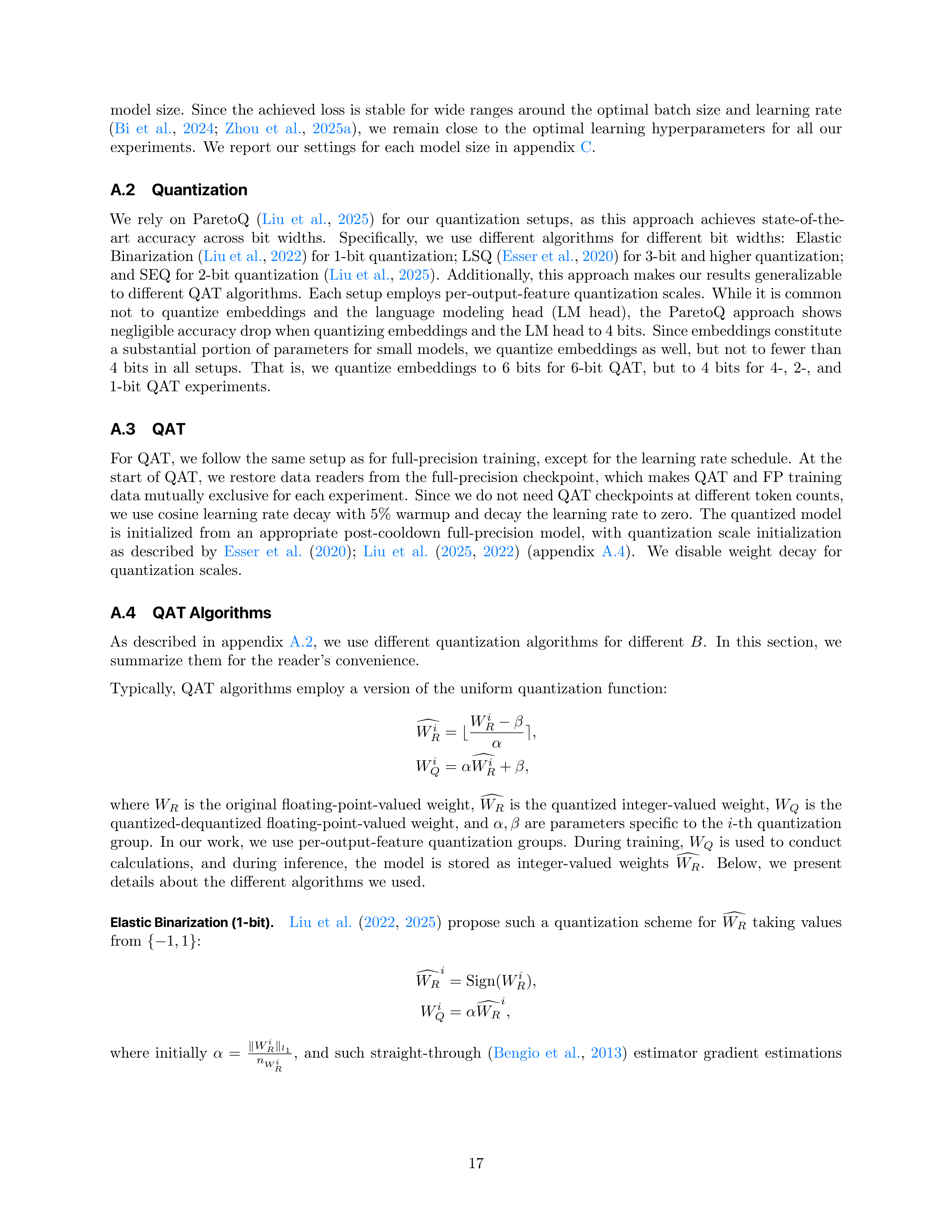
model
size.
Since
the
achieved
loss
is
stable
for
wide
ranges
around
the
optimal
batch
size
and
learning
rate
(
Bi
et
al.
,
2024
;
Zhou
et
al.
,
2025a
),
we
remain
close
to
the
optimal
learning
hyperparameters
for
all
our
experiments.
We
report
our
settings
for
each
model
size
in
appendix
C
.
A.2
Quantization
We
rely
on
ParetoQ
(
Liu
et
al.
,
2025
)
for
our
quantization
setups,
as
this
approach
achieves
state-of-the-
art
accuracy
across
bit
widths.
Specifically,
we
use
different
algorithms
for
different
bit
widths:
Elastic
Binarization (
Liu et al.
,
2022
) for 1-bit quantization; LSQ (
Esser et al.
,
2020
) for 3-bit and higher quantization;
and SEQ for 2-bit quantization (
Liu et al.
,
2025
).
Additionally, this approach makes our results generalizable
to different QAT algorithms.
Each setup employs per-output-feature quantization scales.
While it is common
not
to
quantize
embeddings
and
the
language
modeling
head
(LM
head),
the
ParetoQ
approach
shows
negligible accuracy drop when quantizing embeddings and the LM head to 4 bits.
Since embeddings constitute
a
substantial
portion
of
parameters
for
small
models,
we
quantize
embeddings
as
well,
but
not
to
fewer
than
4
bits
in
all
setups.
That
is,
we
quantize
embeddings
to
6
bits
for
6-bit
QAT,
but
to
4
bits
for
4-,
2-,
and
1-bit
QAT
experiments.
A.3
QAT
For QAT, we follow the same setup as for full-precision training, except for the learning rate schedule.
At the
start
of
QAT,
we
restore
data
readers
from
the
full-precision
checkpoint,
which
makes
QAT
and
FP
training
data mutually exclusive for each experiment.
Since we do not need QAT checkpoints at different token counts,
we use cosine learning rate decay with 5% warmup and decay the learning rate to zero.
The quantized model
is
initialized
from
an
appropriate
post-cooldown
full-precision
model,
with
quantization
scale
initialization
as
described
by
Esser
et
al.
(
2020
);
Liu
et
al.
(
2025
,
2022
)
(appendix
A.4
).
We
disable
weight
decay
for
quantization
scales.
A.4
QAT Algorithms
As
described
in
appendix
A.2
,
we
use
different
quantization
algorithms
for
different
B
.
In
this
section,
we
summarize
them
for
the
reader’s
convenience.
Typically,
QAT
algorithms
employ
a
version
of
the
uniform
quantization
function:
d
W
i
R
=
⌊
W
i
R
−
β
α
⌉
,
W
i
Q
=
α
d
W
i
R
+
β,
where
W
R
is
the
original
floating-point-valued
weight,
d
W
R
is
the
quantized
integer-valued
weight,
W
Q
is
the
quantized-dequantized
floating-point-valued
weight,
and
α, β
are parameters specific
to the
i
-th
quantization
group.
In
our
work,
we
use
per-output-feature
quantization
groups.
During
training,
W
Q
is
used
to
conduct
calculations,
and
during
inference,
the
model
is
stored
as
integer-valued
weights
d
W
R
.
Below,
we
present
details
about
the
different
algorithms
we
used.
Elastic Binarization (1-bit).
Liu
et
al.
(
2022
,
2025
)
propose
such
a
quantization
scheme
for
d
W
R
taking
values
from
{−
1
,
1
}
:
d
W
R
i
=
Sign
(
W
i
R
)
,
W
i
Q
=
α
d
W
R
i
,
where
initially
α
=
∥
W
i
R
∥
l
1
n
W i
R
,
and
such
straight-through
(
Bengio
et
al.
,
2013
)
estimator
gradient
estimations
17
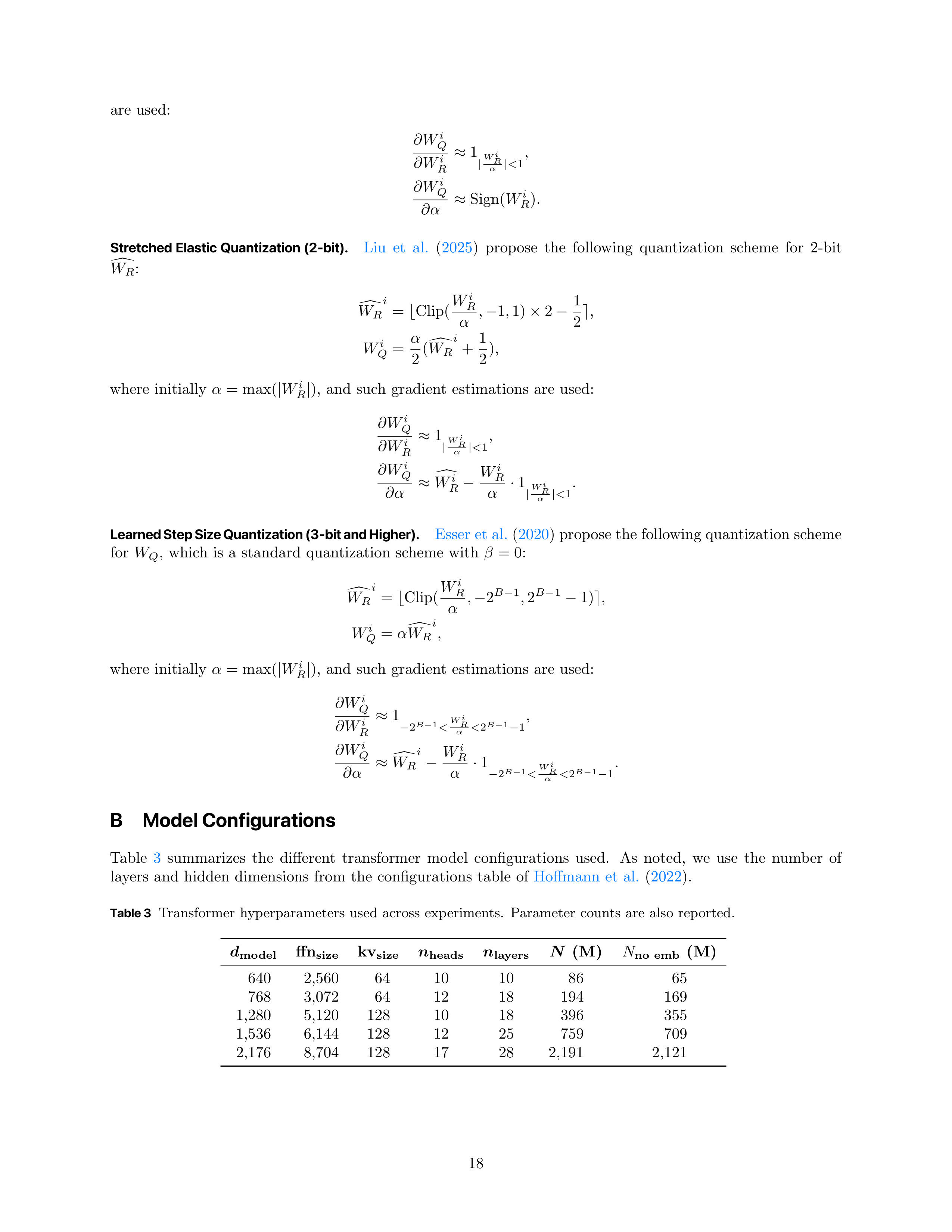
are
used:
∂W
i
Q
∂W
i
R
≈
1
|
W
i
R
α
|
<
1
,
∂W
i
Q
∂α
≈
Sign
(
W
i
R
)
.
Stretched Elastic Quantization (2-bit).
Liu
et
al.
(
2025
)
propose
the
following
quantization
scheme
for
2-bit
d
W
R
:
d
W
R
i
=
⌊
Clip
(
W
i
R
α
,
−
1
,
1)
×
2
−
1
2
⌉
,
W
i
Q
=
α
2
(
d
W
R
i
+
1
2
)
,
where
initially
α
= max(
|
W
i
R
|
)
,
and
such
gradient
estimations
are
used:
∂W
i
Q
∂W
i
R
≈
1
|
W
i
R
α
|
<
1
,
∂W
i
Q
∂α
≈
d
W
i
R
−
W
i
R
α
·
1
|
W
i
R
α
|
<
1
.
Learned Step Size Quantization (3-bit and Higher).
Esser et al.
(
2020
) propose the following quantization scheme
for
W
Q
,
which
is
a
standard
quantization
scheme
with
β
= 0
:
d
W
R
i
=
⌊
Clip
(
W
i
R
α
,
−
2
B
−
1
,
2
B
−
1
−
1)
⌉
,
W
i
Q
=
α
d
W
R
i
,
where
initially
α
= max(
|
W
i
R
|
)
,
and
such
gradient
estimations
are
used:
∂W
i
Q
∂W
i
R
≈
1
−
2
B
−
1
<
W
i
R
α
<
2
B
−
1
−
1
,
∂W
i
Q
∂α
≈
d
W
R
i
−
W
i
R
α
·
1
−
2
B
−
1
<
W
i
R
α
<
2
B
−
1
−
1
.
B
Model Configurations
Table
3
summarizes
the
different
transformer
model
configurations
used.
As
noted,
we
use
the
number
of
layers
and
hidden
dimensions
from
the
configurations
table
of
Hoffmann
et
al.
(
2022
).
Table 3
Transformer
hyperparameters
used
across
experiments.
Parameter
counts
are
also
reported.
d
model
ffn
size
kv
size
n
heads
n
layers
N
(M)
N
no
emb
(M)
640
2
,
560
64
10
10
86
65
768
3
,
072
64
12
18
194
169
1
,
280
5
,
120
128
10
18
396
355
1
,
536
6
,
144
128
12
25
759
709
2
,
176
8
,
704
128
17
28
2
,
191
2
,
121
18
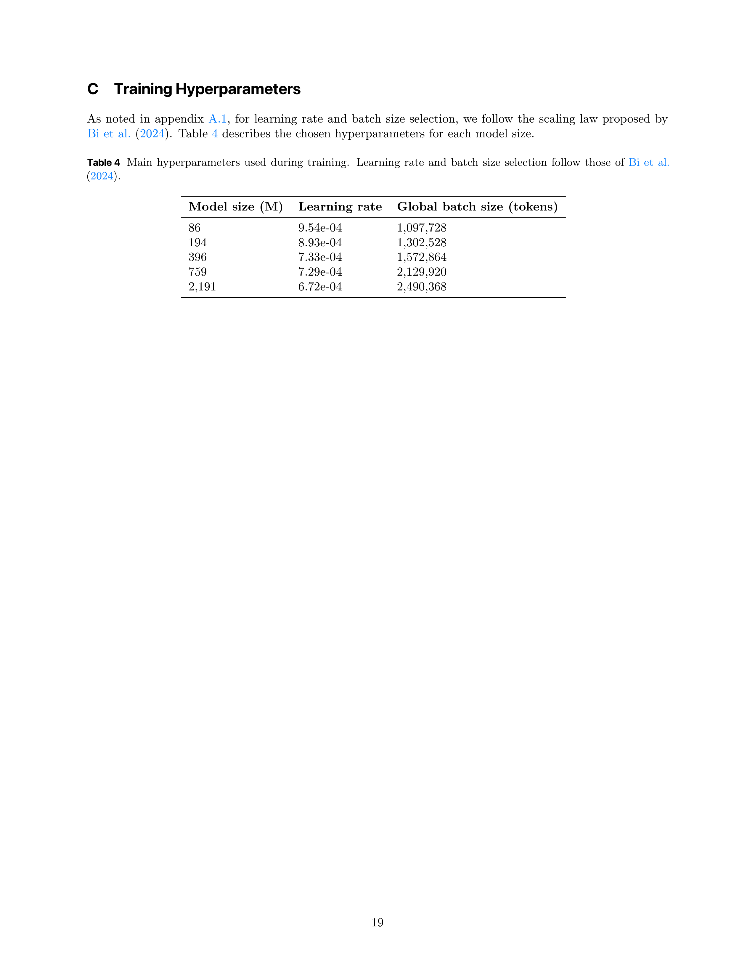
C
Training Hyperparameters
As
noted
in
appendix
A.1
,
for
learning
rate
and
batch
size
selection,
we
follow
the
scaling
law
proposed
by
Bi
et
al.
(
2024
).
Table
4
describes
the
chosen
hyperparameters
for
each
model
size.
Table 4
Main
hyperparameters
used
during
training.
Learning
rate
and
batch
size
selection
follow
those
of
Bi
et
al.
(
2024
).
Model
size
(M)
Learning
rate
Global
batch
size
(tokens)
86
9.54e-04
1,097,728
194
8.93e-04
1,302,528
396
7.33e-04
1,572,864
759
7.29e-04
2,129,920
2,191
6.72e-04
2,490,368
19
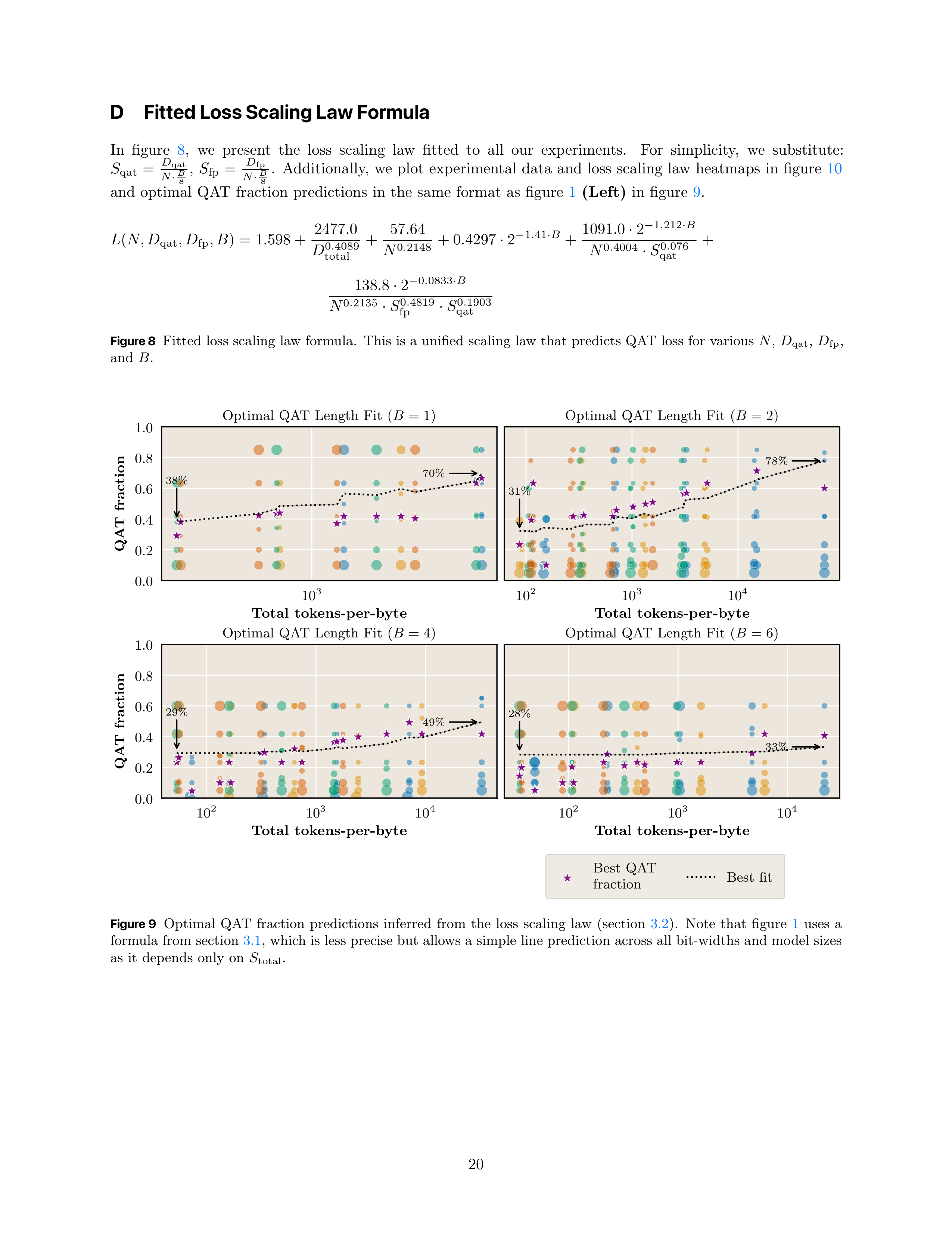
D
Fitted Loss Scaling Law Formula
In
figure
8
,
we
present
the
loss
scaling
law
fitted
to
all
our
experiments.
For
simplicity,
we
substitute:
S
qat
=
D
qat
N
·
B
8
,
S
fp
=
D
fp
N
·
B
8
.
Additionally,
we
plot
experimental
data
and
loss
scaling
law
heatmaps
in
figure
10
and
optimal
QAT
fraction
predictions
in
the
same
format
as
figure
1
(Left)
in
figure
9
.
L
(
N, D
qat
, D
fp
, B
) = 1
.
598 +
2477
.
0
D
0
.
4089
total
+
57
.
64
N
0
.
2148
+ 0
.
4297
·
2
−
1
.
41
·
B
+
1091
.
0
·
2
−
1
.
212
·
B
N
0
.
4004
·
S
0
.
076
qat
+
138
.
8
·
2
−
0
.
0833
·
B
N
0
.
2135
·
S
0
.
4819
fp
·
S
0
.
1903
qat
Figure 8
Fitted
loss
scaling
law
formula.
This
is
a
unified
scaling
law
that
predicts
QAT
loss
for
various
N
,
D
qat
,
D
fp
,
and
B
.
10
3
Total
tokens-per-byte
0
.
0
0
.
2
0
.
4
0
.
6
0
.
8
1
.
0
QAT
fraction
38%
70%
Optimal
QAT
Length
Fit
(
B
= 1
)
10
2
10
3
10
4
Total
tokens-per-byte
31%
78%
Optimal
QAT
Length
Fit
(
B
= 2
)
10
2
10
3
10
4
Total
tokens-per-byte
0
.
0
0
.
2
0
.
4
0
.
6
0
.
8
1
.
0
QAT
fraction
29%
49%
Optimal
QAT
Length
Fit
(
B
= 4
)
10
2
10
3
10
4
Total
tokens-per-byte
28%
33%
Optimal
QAT
Length
Fit
(
B
= 6
)
Best
QAT
fraction
Best
fit
Figure 9
Optimal
QAT
fraction
predictions
inferred
from
the
loss
scaling
law
(section
3.2
).
Note
that
figure
1
uses
a
formula
from
section
3.1
,
which
is
less
precise
but
allows
a
simple
line
prediction
across
all
bit-widths
and
model
sizes
as
it
depends
only
on
S
total
.
20
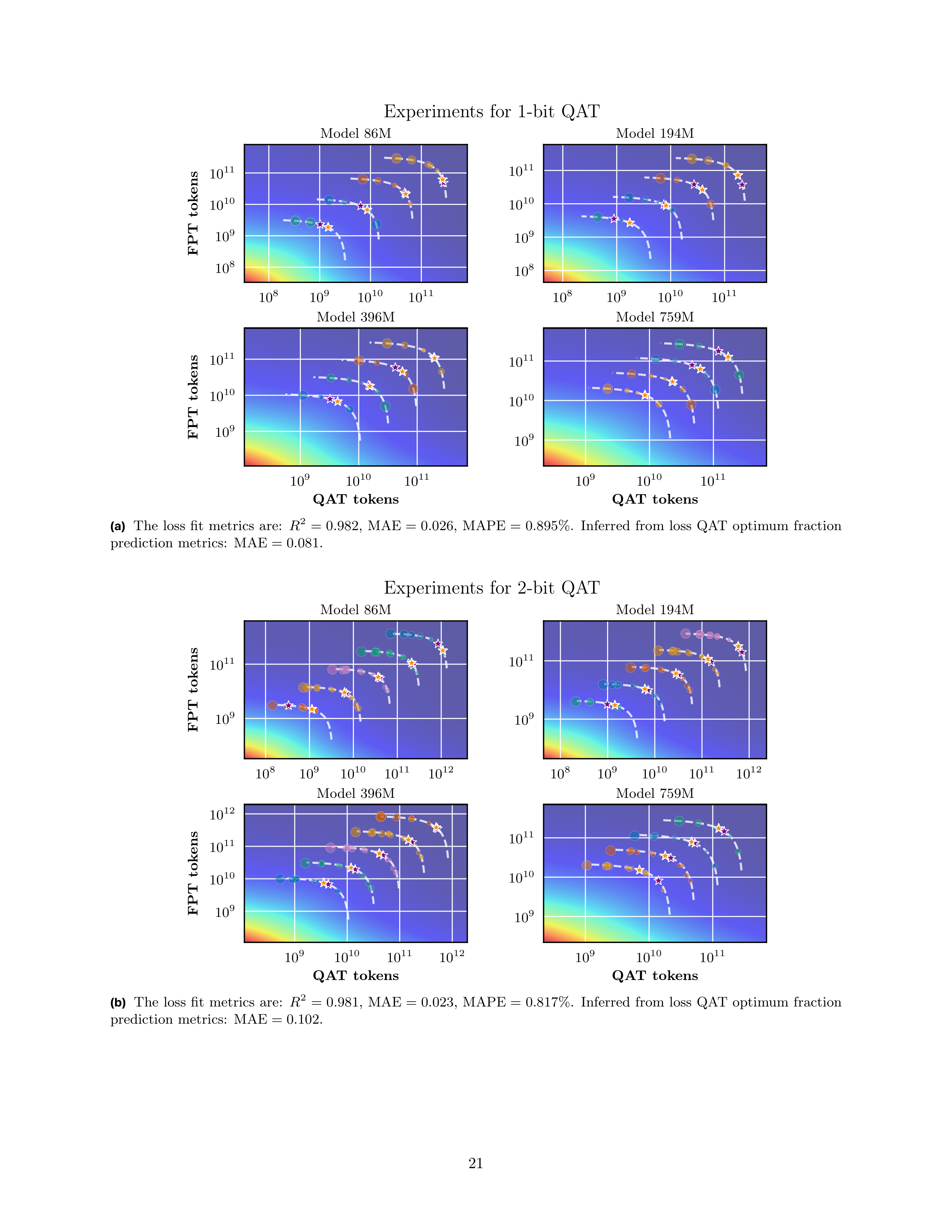
10
8
10
9
10
10
10
11
10
8
10
9
10
10
10
11
FPT
tokens
Model
86M
10
8
10
9
10
10
10
11
10
8
10
9
10
10
10
11
Model
194M
10
9
10
10
10
11
QAT
tokens
10
9
10
10
10
11
FPT
tokens
Model
396M
10
9
10
10
10
11
QAT
tokens
10
9
10
10
10
11
Model
759M
Experiments
for
1-bit
QAT
(a)
The
loss
fit
metrics
are:
R
2
=
0
.
982
,
MAE
=
0
.
026
,
MAPE
=
0
.
895%
.
Inferred
from
loss
QAT
optimum
fraction
prediction
metrics:
MAE
= 0
.
081
.
10
8
10
9
10
10
10
11
10
12
10
9
10
11
FPT
tokens
Model
86M
10
8
10
9
10
10
10
11
10
12
10
9
10
11
Model
194M
10
9
10
10
10
11
10
12
QAT
tokens
10
9
10
10
10
11
10
12
FPT
tokens
Model
396M
10
9
10
10
10
11
QAT
tokens
10
9
10
10
10
11
Model
759M
Experiments
for
2-bit
QAT
(b)
The
loss
fit
metrics
are:
R
2
=
0
.
981
,
MAE
= 0
.
023
,
MAPE
=
0
.
817%
.
Inferred
from
loss
QAT
optimum
fraction
prediction
metrics:
MAE
= 0
.
102
.
21
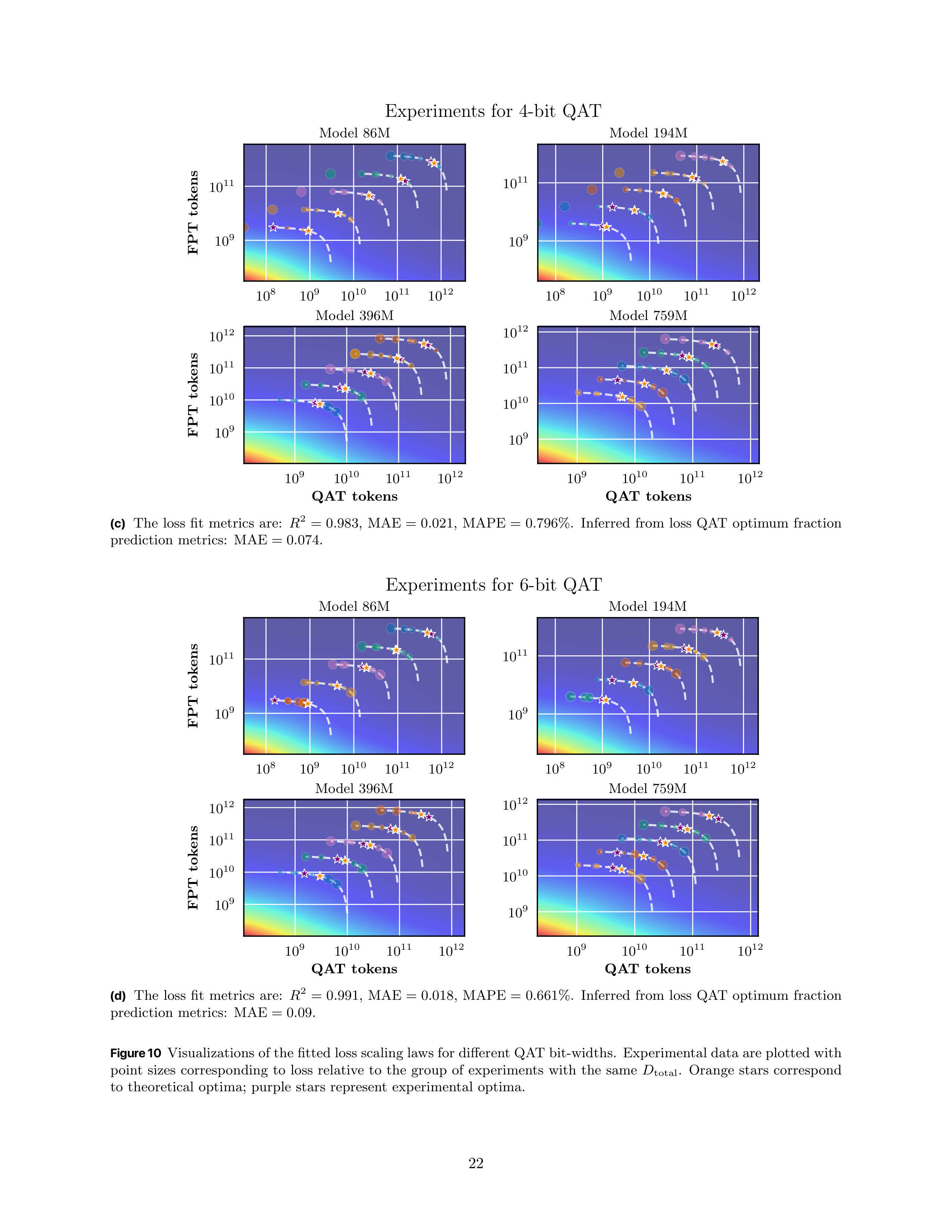

10
8
10
9
10
10
10
11
10
12
10
9
10
11
FPT
tokens
Model
86M
10
8
10
9
10
10
10
11
10
12
10
9
10
11
Model
194M
10
9
10
10
10
11
10
12
QAT
tokens
10
9
10
10
10
11
10
12
FPT
tokens
Model
396M
10
9
10
10
10
11
10
12
QAT
tokens
10
9
10
10
10
11
10
12
Model
759M
Experiments
for
4-bit
QAT
(c)
The
loss
fit
metrics
are:
R
2
=
0
.
983
,
MAE
=
0
.
021
,
MAPE
=
0
.
796%
.
Inferred
from
loss
QAT
optimum
fraction
prediction
metrics:
MAE
= 0
.
074
.
10
8
10
9
10
10
10
11
10
12
10
9
10
11
FPT
tokens
Model
86M
10
8
10
9
10
10
10
11
10
12
10
9
10
11
Model
194M
10
9
10
10
10
11
10
12
QAT
tokens
10
9
10
10
10
11
10
12
FPT
tokens
Model
396M
10
9
10
10
10
11
10
12
QAT
tokens
10
9
10
10
10
11
10
12
Model
759M
Experiments
for
6-bit
QAT
(d)
The
loss
fit
metrics
are:
R
2
=
0
.
991
,
MAE
= 0
.
018
,
MAPE
= 0
.
661%
.
Inferred
from
loss
QAT
optimum
fraction
prediction
metrics:
MAE
= 0
.
09
.
Figure 10
Visualizations of the fitted loss scaling laws for different QAT bit-widths.
Experimental data are plotted with
point
sizes
corresponding
to
loss
relative
to
the
group
of
experiments
with
the
same
D
total
.
Orange
stars
correspond
to
theoretical
optima;
purple
stars
represent
experimental
optima.
22
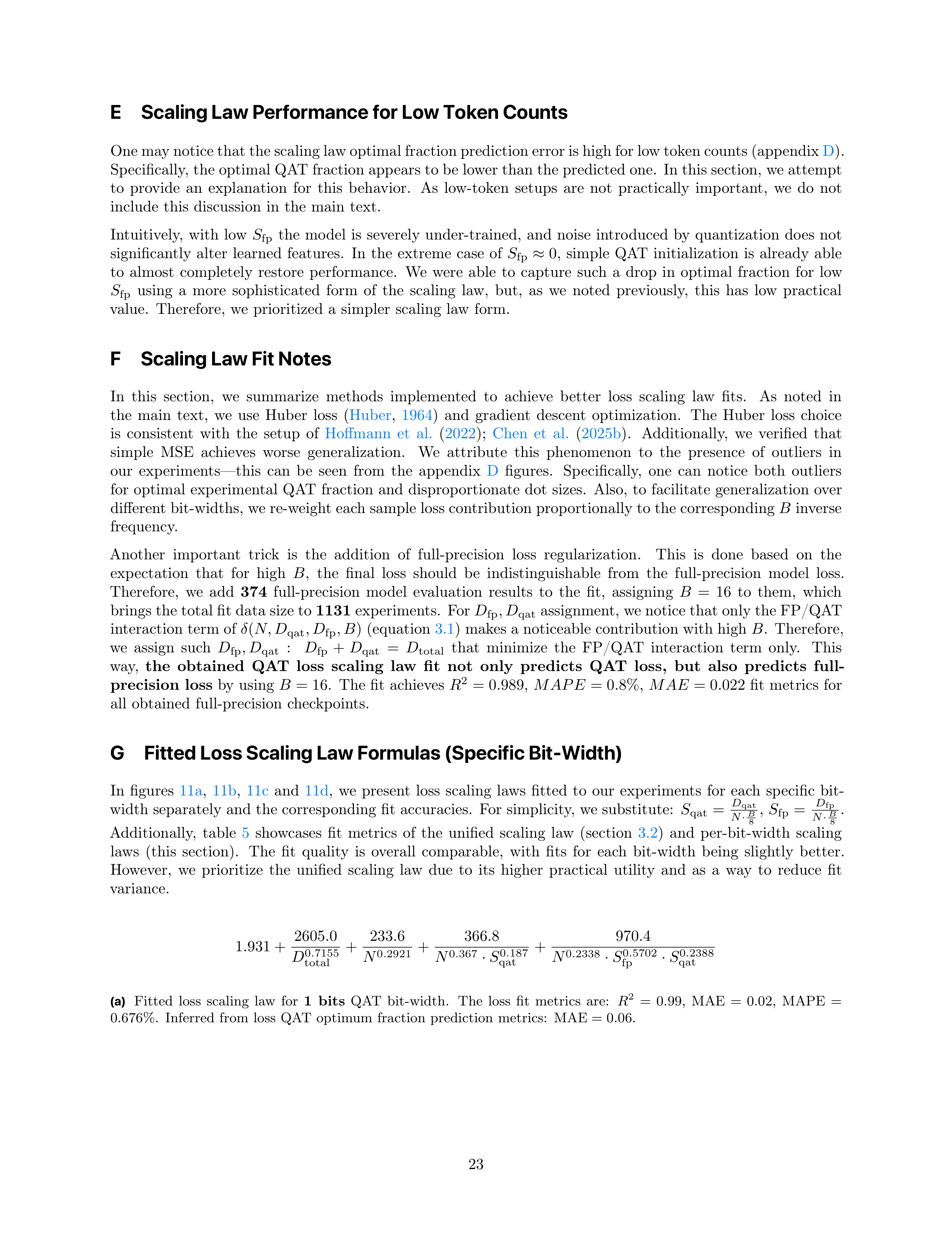
E
Scaling Law Performance for Low Token Counts
One may notice that the scaling law optimal fraction prediction error is high for low token counts (appendix
D
).
Specifically, the optimal QAT fraction appears to be lower than the predicted one.
In this section, we attempt
to
provide
an
explanation
for
this
behavior.
As
low-token
setups
are
not
practically
important,
we
do
not
include
this
discussion
in
the
main
text.
Intuitively,
with
low
S
fp
the
model
is
severely
under-trained,
and
noise
introduced
by
quantization
does
not
significantly
alter
learned
features.
In
the
extreme
case
of
S
fp
≈
0
,
simple
QAT
initialization
is
already
able
to
almost
completely
restore
performance.
We
were
able
to
capture
such
a
drop
in
optimal
fraction
for
low
S
fp
using
a
more
sophisticated
form
of
the
scaling
law,
but,
as
we
noted
previously,
this
has
low
practical
value.
Therefore,
we
prioritized
a
simpler
scaling
law
form.
F
Scaling Law Fit Notes
In
this
section,
we
summarize
methods
implemented
to
achieve
better
loss
scaling
law
fits.
As
noted
in
the
main
text,
we
use
Huber
loss
(
Huber
,
1964
)
and
gradient
descent
optimization.
The
Huber
loss
choice
is
consistent
with
the
setup
of
Hoffmann
et
al.
(
2022
);
Chen
et
al.
(
2025b
).
Additionally,
we
verified
that
simple
MSE
achieves
worse
generalization.
We
attribute
this
phenomenon
to
the
presence
of
outliers
in
our
experiments—this
can
be
seen
from
the
appendix
D
figures.
Specifically,
one
can
notice
both
outliers
for
optimal
experimental
QAT
fraction
and
disproportionate
dot
sizes.
Also,
to
facilitate
generalization
over
different bit-widths, we re-weight each sample loss contribution proportionally to the corresponding
B
inverse
frequency.
Another
important
trick
is
the
addition
of
full-precision
loss
regularization.
This
is
done
based
on
the
expectation
that
for
high
B
,
the
final
loss
should
be
indistinguishable
from
the
full-precision
model
loss.
Therefore,
we
add
374
full-precision
model
evaluation
results
to
the
fit,
assigning
B
=
16
to
them,
which
brings the total fit data size to
1131
experiments.
For
D
fp
, D
qat
assignment, we notice that only the FP/QAT
interaction term of
δ
(
N, D
qat
, D
fp
, B
)
(equation
3.1
) makes a noticeable contribution with high
B
.
Therefore,
we
assign
such
D
fp
, D
qat
:
D
fp
+
D
qat
=
D
total
that
minimize
the
FP/QAT
interaction
term
only.
This
way,
the
obtained
QAT
loss
scaling
law
fit
not
only
predicts
QAT
loss,
but
also
predicts
full-
precision
loss
by
using
B
= 16
.
The
fit
achieves
R
2
= 0
.
989
,
MAPE
= 0
.
8%
,
MAE
= 0
.
022
fit
metrics
for
all
obtained
full-precision
checkpoints.
G
Fitted Loss Scaling Law Formulas (Specific Bit-Width)
In
figures
11a
,
11b
,
11c
and
11d
,
we
present
loss
scaling
laws
fitted
to
our
experiments
for
each
specific
bit-
width separately and the corresponding fit accuracies.
For simplicity,
we substitute:
S
qat
=
D
qat
N
·
B
8
,
S
fp
=
D
fp
N
·
B
8
.
Additionally,
table
5
showcases
fit
metrics
of
the
unified
scaling
law
(section
3.2
)
and
per-bit-width
scaling
laws
(this
section).
The
fit
quality
is
overall
comparable,
with
fits
for
each
bit-width
being
slightly
better.
However,
we
prioritize
the
unified
scaling
law
due
to
its
higher
practical
utility
and
as
a
way
to
reduce
fit
variance.
1
.
931 +
2605
.
0
D
0
.
7155
total
+
233
.
6
N
0
.
2921
+
366
.
8
N
0
.
367
·
S
0
.
187
qat
+
970
.
4
N
0
.
2338
·
S
0
.
5702
fp
·
S
0
.
2388
qat
(a)
Fitted
loss
scaling
law
for
1
bits
QAT
bit-width.
The
loss
fit
metrics
are:
R
2
=
0
.
99
,
MAE
=
0
.
02
,
MAPE
=
0
.
676%
.
Inferred
from
loss
QAT
optimum
fraction
prediction
metrics:
MAE
= 0
.
06
.
23
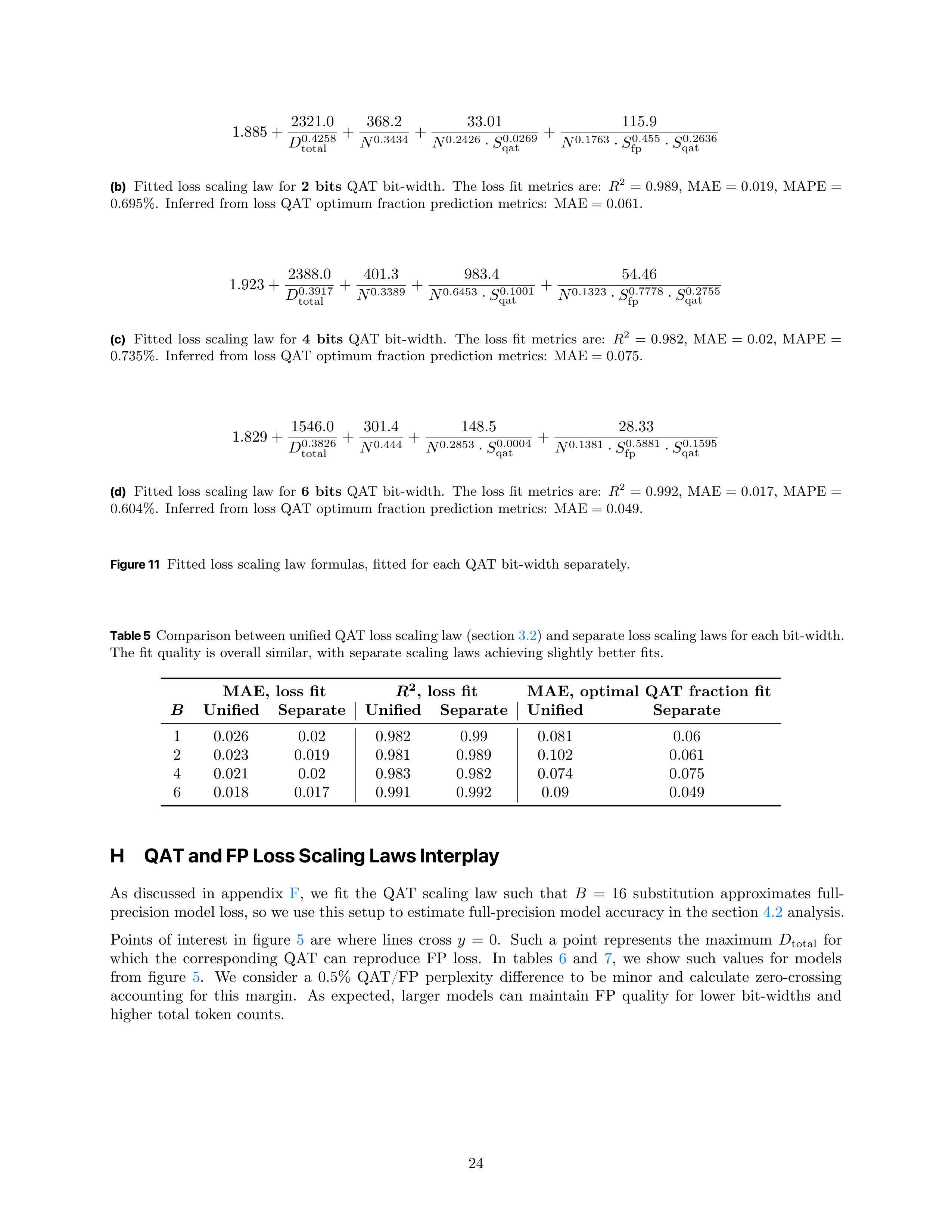
1
.
885 +
2321
.
0
D
0
.
4258
total
+
368
.
2
N
0
.
3434
+
33
.
01
N
0
.
2426
·
S
0
.
0269
qat
+
115
.
9
N
0
.
1763
·
S
0
.
455
fp
·
S
0
.
2636
qat
(b)
Fitted
loss
scaling
law
for
2
bits
QAT
bit-width.
The
loss
fit
metrics
are:
R
2
=
0
.
989
,
MAE
=
0
.
019
,
MAPE
=
0
.
695%
.
Inferred
from
loss
QAT
optimum
fraction
prediction
metrics:
MAE
= 0
.
061
.
1
.
923 +
2388
.
0
D
0
.
3917
total
+
401
.
3
N
0
.
3389
+
983
.
4
N
0
.
6453
·
S
0
.
1001
qat
+
54
.
46
N
0
.
1323
·
S
0
.
7778
fp
·
S
0
.
2755
qat
(c)
Fitted
loss
scaling
law
for
4
bits
QAT
bit-width.
The
loss
fit
metrics
are:
R
2
=
0
.
982
,
MAE
=
0
.
02
,
MAPE
=
0
.
735%
.
Inferred
from
loss
QAT
optimum
fraction
prediction
metrics:
MAE
= 0
.
075
.
1
.
829 +
1546
.
0
D
0
.
3826
total
+
301
.
4
N
0
.
444
+
148
.
5
N
0
.
2853
·
S
0
.
0004
qat
+
28
.
33
N
0
.
1381
·
S
0
.
5881
fp
·
S
0
.
1595
qat
(d)
Fitted
loss
scaling
law
for
6
bits
QAT
bit-width.
The
loss
fit
metrics
are:
R
2
=
0
.
992
,
MAE
=
0
.
017
,
MAPE
=
0
.
604%
.
Inferred
from
loss
QAT
optimum
fraction
prediction
metrics:
MAE
= 0
.
049
.
Figure 11
Fitted
loss
scaling
law
formulas,
fitted
for
each
QAT
bit-width
separately.
Table 5
Comparison between unified QAT loss scaling law (section
3.2
) and separate loss scaling laws for each bit-width.
The
fit
quality
is
overall
similar,
with
separate
scaling
laws
achieving
slightly
better
fits.
MAE,
loss
fit
R
2
,
loss
fit
MAE,
optimal
QAT
fraction
fit
B
Unified
Separate
Unified
Separate
Unified
Separate
1
0.026
0.02
0.982
0.99
0.081
0.06
2
0.023
0.019
0.981
0.989
0.102
0.061
4
0.021
0.02
0.983
0.982
0.074
0.075
6
0.018
0.017
0.991
0.992
0.09
0.049
H
QAT and FP Loss Scaling Laws Interplay
As
discussed
in
appendix
F
,
we
fit
the
QAT
scaling
law
such
that
B
=
16
substitution
approximates
full-
precision model loss, so we use this setup to estimate full-precision model accuracy in the section
4.2
analysis.
Points
of
interest
in
figure
5
are
where
lines
cross
y
=
0
.
Such
a
point
represents
the
maximum
D
total
for
which
the
corresponding
QAT
can
reproduce
FP
loss.
In
tables
6
and
7
,
we
show
such
values
for
models
from
figure
5
.
We
consider
a
0.5%
QAT/FP
perplexity
difference
to
be
minor
and
calculate
zero-crossing
accounting
for
this
margin.
As
expected,
larger
models
can
maintain
FP
quality
for
lower
bit-widths
and
higher
total
token
counts.
24
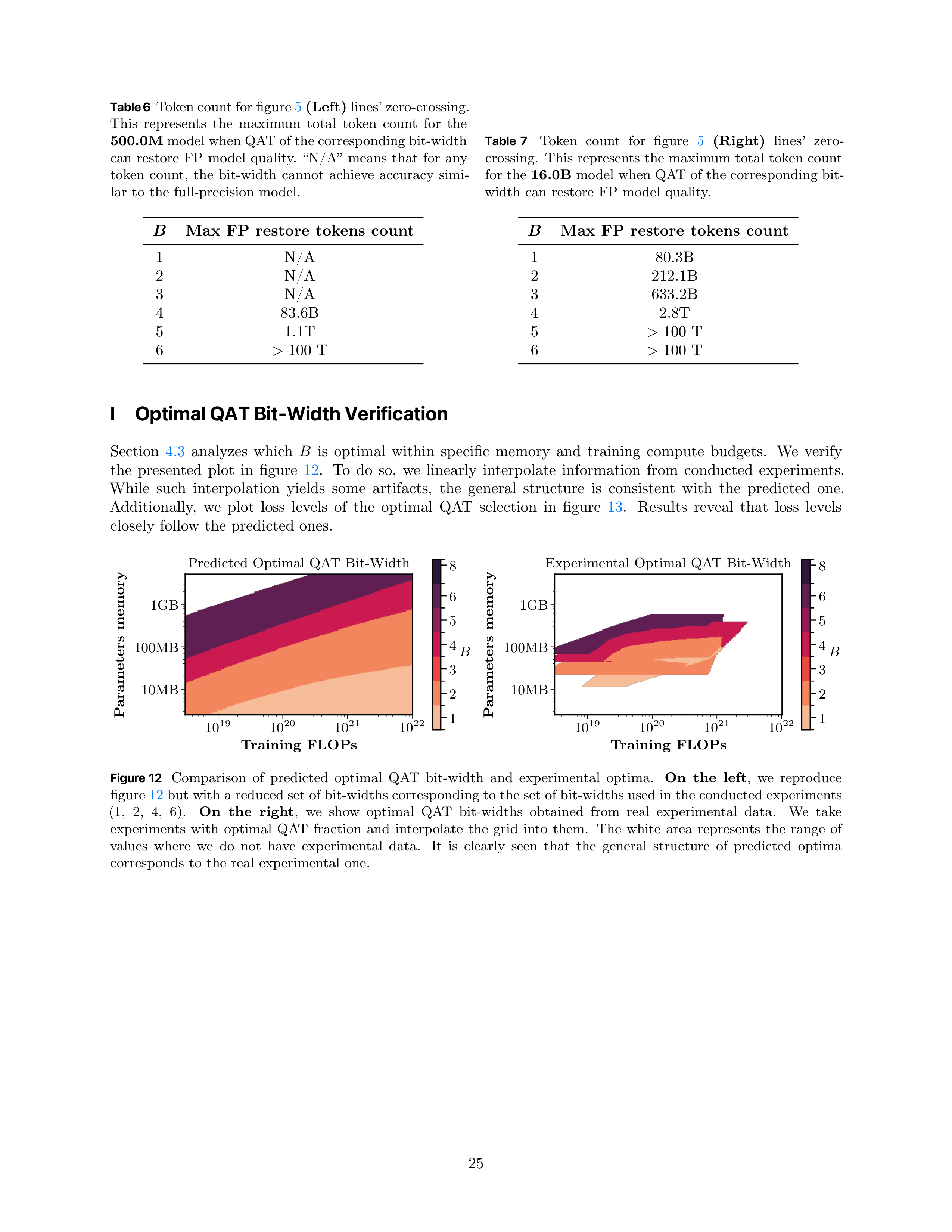


Table6
Token count for figure
5
(Left)
lines’ zero-crossing.
This
represents
the
maximum
total
token
count
for
the
500.0M
model when QAT of the corresponding bit-width
can
restore
FP
model
quality.
“N/A”
means
that
for
any
token
count,
the
bit-width
cannot
achieve
accuracy
simi-
lar
to
the
full-precision
model.
B
Max
FP
restore
tokens
count
1
N/A
2
N/A
3
N/A
4
83.6B
5
1.1T
6
>
100
T
Table
7
Token
count
for
figure
5
(Right)
lines’
zero-
crossing.
This
represents
the
maximum
total
token
count
for
the
16.0B
model
when
QAT
of
the
corresponding
bit-
width
can
restore
FP
model
quality.
B
Max
FP
restore
tokens
count
1
80.3B
2
212.1B
3
633.2B
4
2.8T
5
>
100
T
6
>
100
T
I
Optimal QAT Bit-Width Verification
Section
4.3
analyzes
which
B
is
optimal
within
specific
memory
and
training
compute
budgets.
We
verify
the
presented
plot
in
figure
12
.
To
do
so,
we
linearly
interpolate
information
from
conducted
experiments.
While
such
interpolation
yields
some
artifacts,
the
general
structure
is
consistent
with
the
predicted
one.
Additionally,
we
plot
loss
levels
of
the
optimal
QAT
selection
in
figure
13
.
Results
reveal
that
loss
levels
closely
follow
the
predicted
ones.
10
19
10
20
10
21
10
22
Training
FLOPs
10MB
100MB
1GB
Parameters
memory
Predicted
Optimal
QAT
Bit-Width
1
2
3
4
5
6
8
B
10
19
10
20
10
21
10
22
Training
FLOPs
10MB
100MB
1GB
Parameters
memory
Experimental
Optimal
QAT
Bit-Width
1
2
3
4
5
6
8
B
Figure 12
Comparison
of
predicted
optimal
QAT
bit-width
and
experimental
optima.
On
the
left
,
we
reproduce
figure
12
but with a reduced set of bit-widths corresponding to the set of bit-widths used in the conducted experiments
(1,
2,
4,
6).
On
the
right
,
we
show
optimal
QAT
bit-widths
obtained
from
real
experimental
data.
We
take
experiments
with
optimal
QAT
fraction
and
interpolate
the
grid
into
them.
The
white
area
represents
the
range
of
values
where
we
do
not
have
experimental
data.
It
is
clearly
seen
that
the
general
structure
of
predicted
optima
corresponds
to
the
real
experimental
one.
25
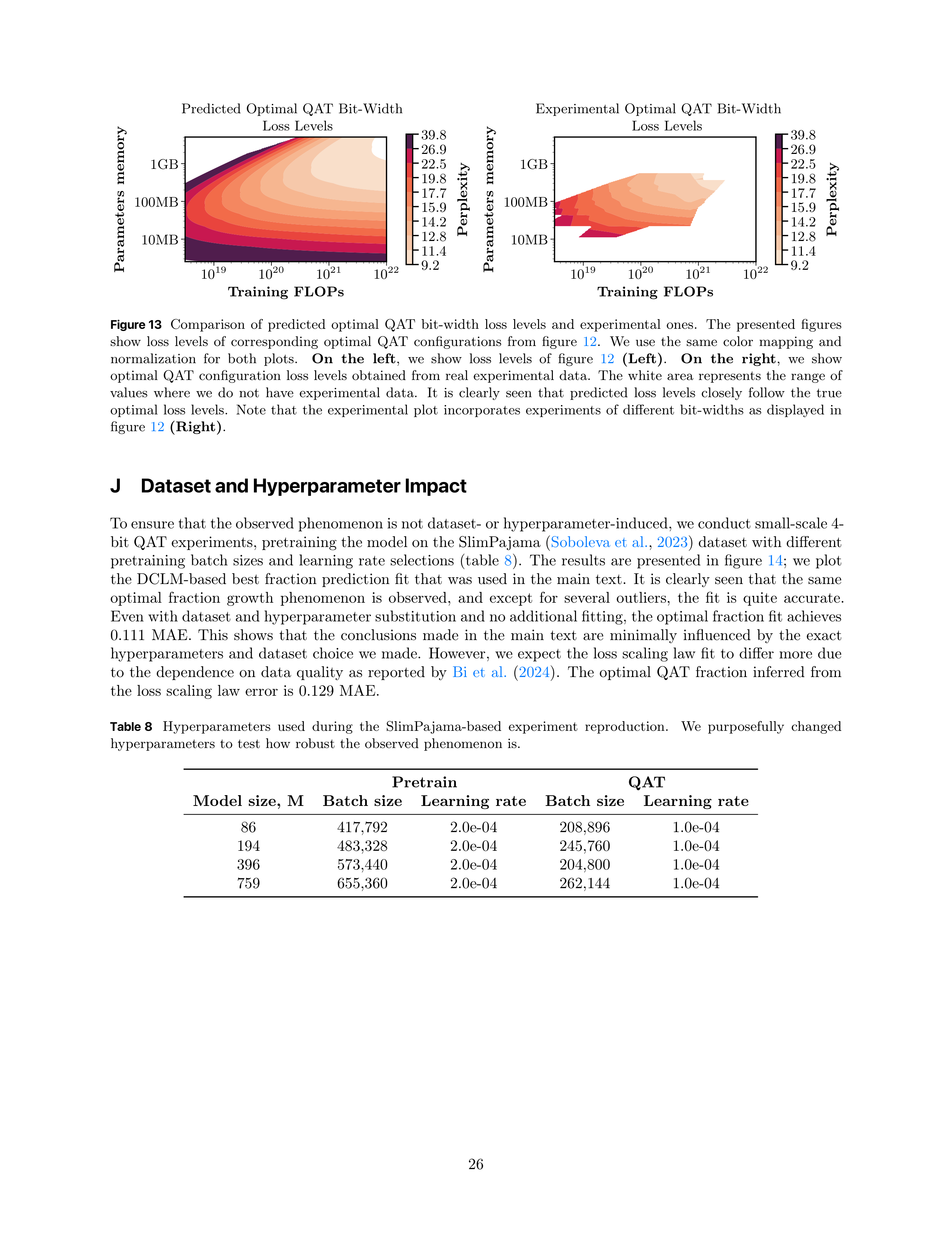
10
19
10
20
10
21
10
22
Training
FLOPs
10MB
100MB
1GB
Parameters
memory
Predicted
Optimal
QAT
Bit-Width
Loss
Levels
9.2
11.4
12.8
14.2
15.9
17.7
19.8
22.5
26.9
39.8
Perplexity
10
19
10
20
10
21
10
22
Training
FLOPs
10MB
100MB
1GB
Parameters
memory
Experimental
Optimal
QAT
Bit-Width
Loss
Levels
9.2
11.4
12.8
14.2
15.9
17.7
19.8
22.5
26.9
39.8
Perplexity
Figure 13
Comparison
of
predicted
optimal
QAT
bit-width
loss
levels
and
experimental
ones.
The
presented
figures
show
loss
levels
of
corresponding
optimal
QAT
configurations
from
figure
12
.
We
use
the
same
color
mapping
and
normalization
for
both
plots.
On
the
left
,
we
show
loss
levels
of
figure
12
(Left)
.
On
the
right
,
we
show
optimal
QAT
configuration
loss
levels
obtained
from
real
experimental
data.
The
white
area
represents
the
range
of
values
where
we
do
not
have
experimental
data.
It
is
clearly
seen
that
predicted
loss
levels
closely
follow
the
true
optimal
loss
levels.
Note
that
the
experimental
plot
incorporates
experiments
of
different
bit-widths
as
displayed
in
figure
12
(Right)
.
J
Dataset and Hyperparameter Impact
To ensure that the observed phenomenon is not dataset- or hyperparameter-induced, we conduct small-scale 4-
bit QAT experiments, pretraining the model on the SlimPajama (
Soboleva et al.
,
2023
) dataset with different
pretraining
batch
sizes
and
learning
rate
selections
(table
8
).
The
results
are
presented
in
figure
14
;
we
plot
the
DCLM-based
best
fraction
prediction
fit
that
was
used
in
the
main
text.
It
is
clearly
seen
that
the
same
optimal
fraction
growth
phenomenon
is
observed,
and
except
for
several
outliers,
the
fit
is
quite
accurate.
Even with dataset and hyperparameter substitution and no additional fitting, the optimal fraction fit achieves
0.111
MAE.
This
shows
that
the
conclusions
made
in
the
main
text
are
minimally
influenced
by
the
exact
hyperparameters
and
dataset
choice
we
made.
However,
we
expect
the
loss
scaling
law
fit
to
differ
more
due
to
the
dependence
on
data
quality
as
reported
by
Bi
et
al.
(
2024
).
The
optimal
QAT
fraction
inferred
from
the
loss
scaling
law
error
is
0.129
MAE.
Table 8
Hyperparameters
used
during
the
SlimPajama-based
experiment
reproduction.
We
purposefully
changed
hyperparameters
to
test
how
robust
the
observed
phenomenon
is.
Pretrain
QAT
Model
size,
M
Batch
size
Learning
rate
Batch
size
Learning
rate
86
417,792
2.0e-04
208,896
1.0e-04
194
483,328
2.0e-04
245,760
1.0e-04
396
573,440
2.0e-04
204,800
1.0e-04
759
655,360
2.0e-04
262,144
1.0e-04
26
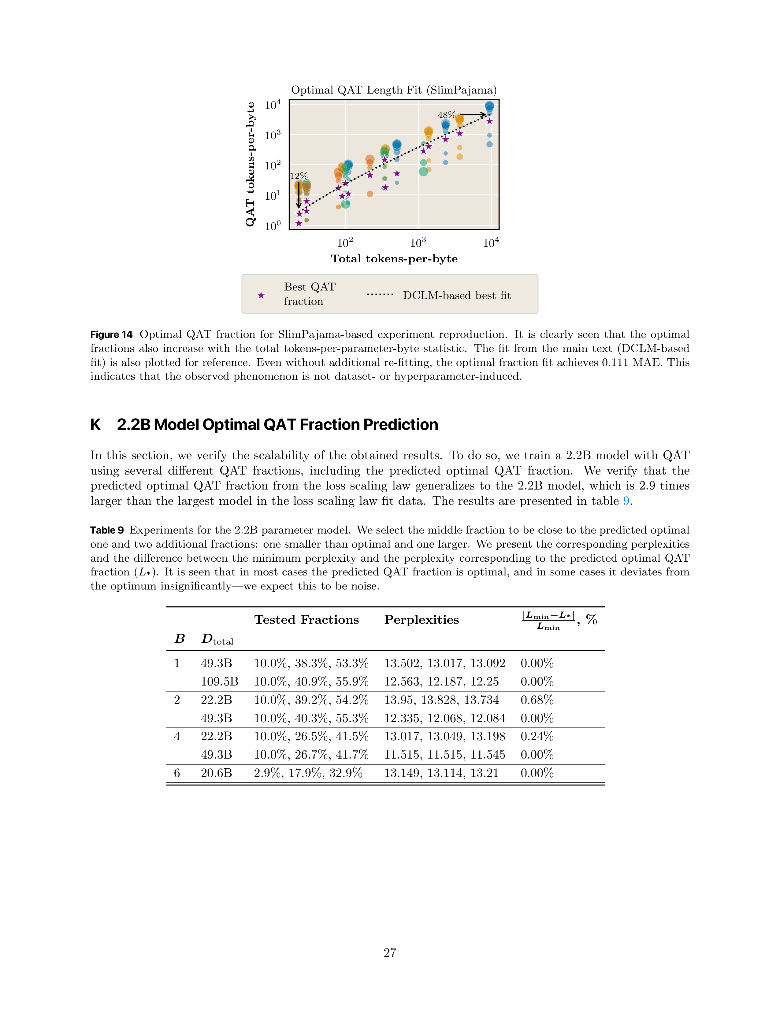
10
2
10
3
10
4
Total
tokens-per-byte
10
0
10
1
10
2
10
3
10
4
QAT
tokens-per-byte
12%
48%
Optimal
QAT
Length
Fit
(SlimPajama)
Best
QAT
fraction
DCLM-based
best
fit
Figure 14
Optimal
QAT
fraction
for
SlimPajama-based
experiment
reproduction.
It
is
clearly
seen
that
the
optimal
fractions
also
increase
with
the
total
tokens-per-parameter-byte
statistic.
The
fit
from
the
main
text
(DCLM-based
fit)
is
also
plotted
for
reference.
Even
without
additional
re-fitting,
the
optimal
fraction
fit
achieves
0.111
MAE.
This
indicates
that
the
observed
phenomenon
is
not
dataset-
or
hyperparameter-induced.
K
2.2B Model Optimal QAT Fraction Prediction
In
this
section,
we
verify
the
scalability
of
the
obtained
results.
To
do
so,
we
train
a
2.2B
model
with
QAT
using
several
different
QAT
fractions,
including
the
predicted
optimal
QAT
fraction.
We
verify
that
the
predicted
optimal
QAT
fraction
from
the
loss
scaling
law
generalizes
to
the
2.2B
model,
which
is
2.9
times
larger
than
the
largest
model
in
the
loss
scaling
law
fit
data.
The
results
are
presented
in
table
9
.
Table 9
Experiments
for
the
2.2B
parameter
model.
We
select
the
middle
fraction
to
be
close
to
the
predicted
optimal
one
and
two
additional
fractions:
one
smaller
than
optimal
and
one
larger.
We
present
the
corresponding
perplexities
and
the
difference
between
the
minimum
perplexity
and
the
perplexity
corresponding
to
the
predicted
optimal
QAT
fraction
(
L
*
).
It
is
seen
that
in
most
cases
the
predicted
QAT
fraction
is
optimal,
and
in
some
cases
it
deviates
from
the
optimum
insignificantly—we
expect
this
to
be
noise.
Tested
Fractions
Perplexities
|
L
min
−
L
*
|
L
min
,
%
B
D
total
1
49.3B
10.0%,
38.3%,
53.3%
13.502,
13.017,
13.092
0.00%
109.5B
10.0%,
40.9%,
55.9%
12.563,
12.187,
12.25
0.00%
2
22.2B
10.0%,
39.2%,
54.2%
13.95,
13.828,
13.734
0.68%
49.3B
10.0%,
40.3%,
55.3%
12.335,
12.068,
12.084
0.00%
4
22.2B
10.0%,
26.5%,
41.5%
13.017,
13.049,
13.198
0.24%
49.3B
10.0%,
26.7%,
41.7%
11.515,
11.515,
11.545
0.00%
6
20.6B
2.9%,
17.9%,
32.9%
13.149,
13.114,
13.21
0.00%
27
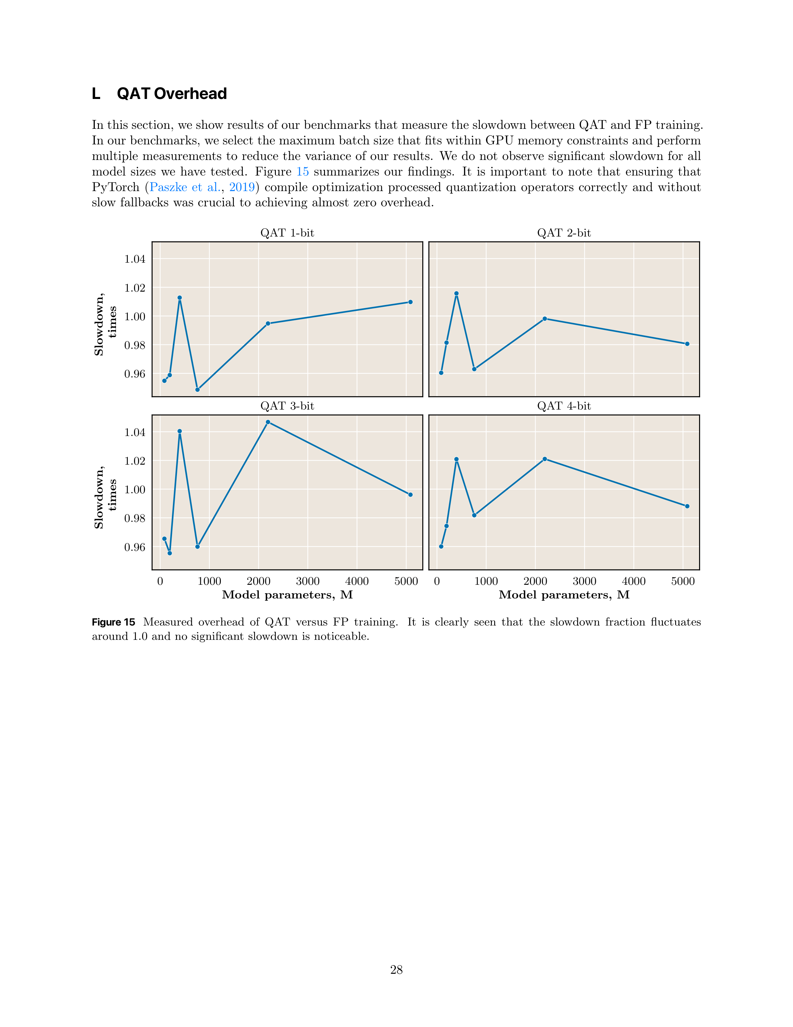
L
QAT Overhead
In this section, we show results of our benchmarks that measure the slowdown between QAT and FP training.
In our benchmarks, we select the maximum batch size that fits within GPU memory constraints and perform
multiple
measurements
to
reduce
the
variance
of
our
results.
We
do
not
observe
significant
slowdown
for
all
model
sizes
we
have
tested.
Figure
15
summarizes
our
findings.
It
is
important
to
note
that
ensuring
that
PyTorch
(
Paszke
et
al.
,
2019
)
compile
optimization
processed
quantization
operators
correctly
and
without
slow
fallbacks
was
crucial
to
achieving
almost
zero
overhead.
0
.
96
0
.
98
1
.
00
1
.
02
1
.
04
Slowdown,
times
QAT
1-bit
QAT
2-bit
0
1000
2000
3000
4000
5000
Model
parameters,
M
0
.
96
0
.
98
1
.
00
1
.
02
1
.
04
Slowdown,
times
QAT
3-bit
0
1000
2000
3000
4000
5000
Model
parameters,
M
QAT
4-bit
Figure 15
Measured
overhead
of
QAT
versus
FP
training.
It
is
clearly
seen
that
the
slowdown
fraction
fluctuates
around
1.0
and
no
significant
slowdown
is
noticeable.
28
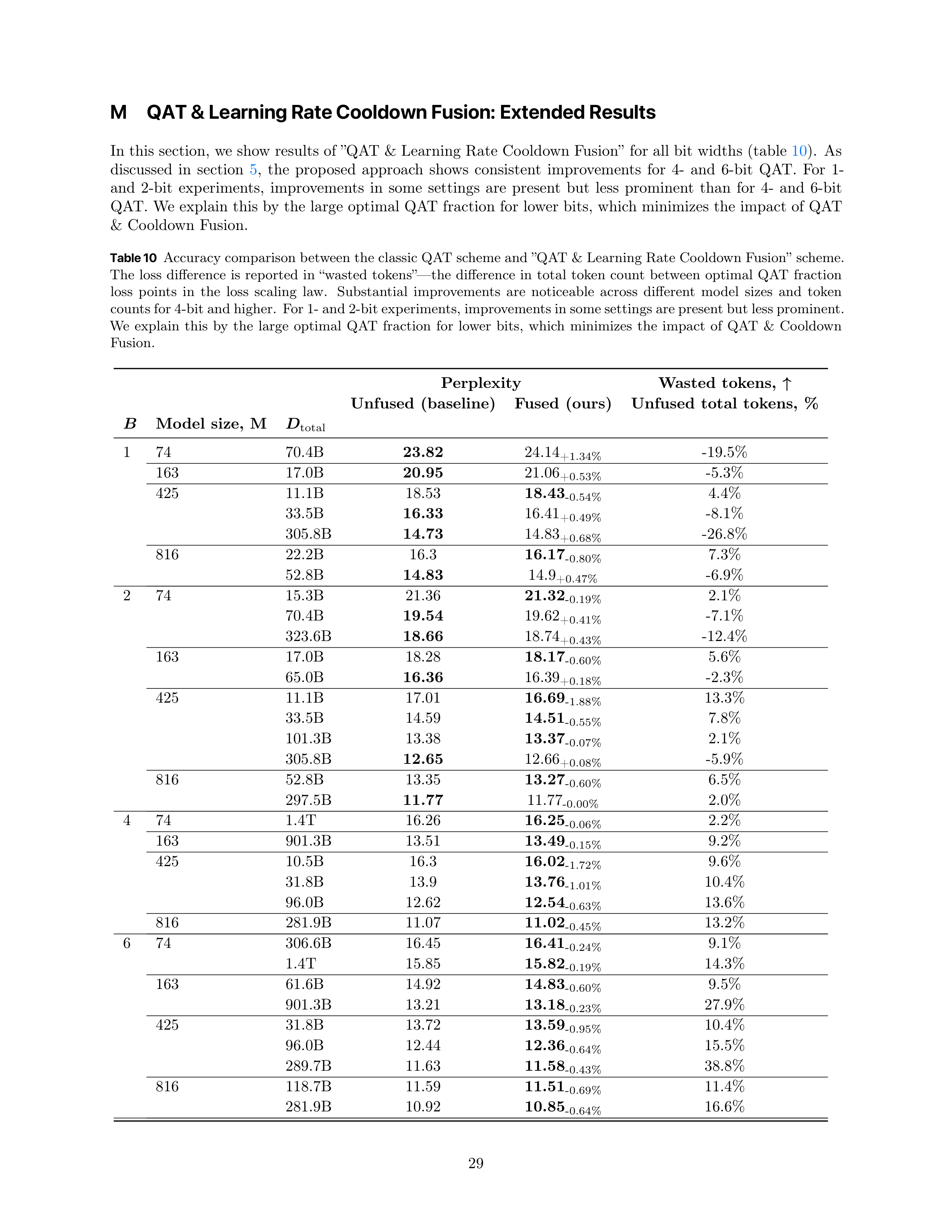
M
QAT & Learning Rate Cooldown Fusion: Extended Results
In
this
section,
we
show
results
of
”QAT
&
Learning
Rate
Cooldown
Fusion”
for
all
bit
widths
(table
10
).
As
discussed
in
section
5
,
the
proposed
approach
shows
consistent
improvements
for
4-
and
6-bit
QAT.
For
1-
and
2-bit
experiments,
improvements
in
some
settings
are
present
but
less
prominent
than
for
4-
and
6-bit
QAT.
We
explain
this
by
the
large
optimal
QAT
fraction
for
lower
bits,
which
minimizes
the
impact
of
QAT
&
Cooldown
Fusion.
Table 10
Accuracy comparison between the classic QAT scheme and ”QAT & Learning Rate Cooldown Fusion”
scheme.
The
loss
difference
is
reported
in
“wasted
tokens”—the
difference
in
total
token
count
between
optimal
QAT
fraction
loss
points
in
the
loss
scaling
law.
Substantial
improvements
are
noticeable
across
different
model
sizes
and
token
counts for 4-bit and higher.
For 1- and 2-bit experiments, improvements in some settings are present but less prominent.
We
explain
this
by
the
large
optimal
QAT
fraction
for
lower
bits,
which
minimizes
the
impact
of
QAT
&
Cooldown
Fusion.
Perplexity
Wasted
tokens,
↑
Unfused
(baseline)
Fused
(ours)
Unfused
total
tokens,
%
B
Model
size,
M
D
total
1
74
70.4B
23.82
24.14
+1.34%
-19.5%
163
17.0B
20.95
21.06
+0.53%
-5.3%
425
11.1B
18.53
18.43
-0.54%
4.4%
33.5B
16.33
16.41
+0.49%
-8.1%
305.8B
14.73
14.83
+0.68%
-26.8%
816
22.2B
16.3
16.17
-0.80%
7.3%
52.8B
14.83
14.9
+0.47%
-6.9%
2
74
15.3B
21.36
21.32
-0.19%
2.1%
70.4B
19.54
19.62
+0.41%
-7.1%
323.6B
18.66
18.74
+0.43%
-12.4%
163
17.0B
18.28
18.17
-0.60%
5.6%
65.0B
16.36
16.39
+0.18%
-2.3%
425
11.1B
17.01
16.69
-1.88%
13.3%
33.5B
14.59
14.51
-0.55%
7.8%
101.3B
13.38
13.37
-0.07%
2.1%
305.8B
12.65
12.66
+0.08%
-5.9%
816
52.8B
13.35
13.27
-0.60%
6.5%
297.5B
11.77
11.77
-0.00%
2.0%
4
74
1.4T
16.26
16.25
-0.06%
2.2%
163
901.3B
13.51
13.49
-0.15%
9.2%
425
10.5B
16.3
16.02
-1.72%
9.6%
31.8B
13.9
13.76
-1.01%
10.4%
96.0B
12.62
12.54
-0.63%
13.6%
816
281.9B
11.07
11.02
-0.45%
13.2%
6
74
306.6B
16.45
16.41
-0.24%
9.1%
1.4T
15.85
15.82
-0.19%
14.3%
163
61.6B
14.92
14.83
-0.60%
9.5%
901.3B
13.21
13.18
-0.23%
27.9%
425
31.8B
13.72
13.59
-0.95%
10.4%
96.0B
12.44
12.36
-0.64%
15.5%
289.7B
11.63
11.58
-0.43%
38.8%
816
118.7B
11.59
11.51
-0.69%
11.4%
281.9B
10.92
10.85
-0.64%
16.6%
29
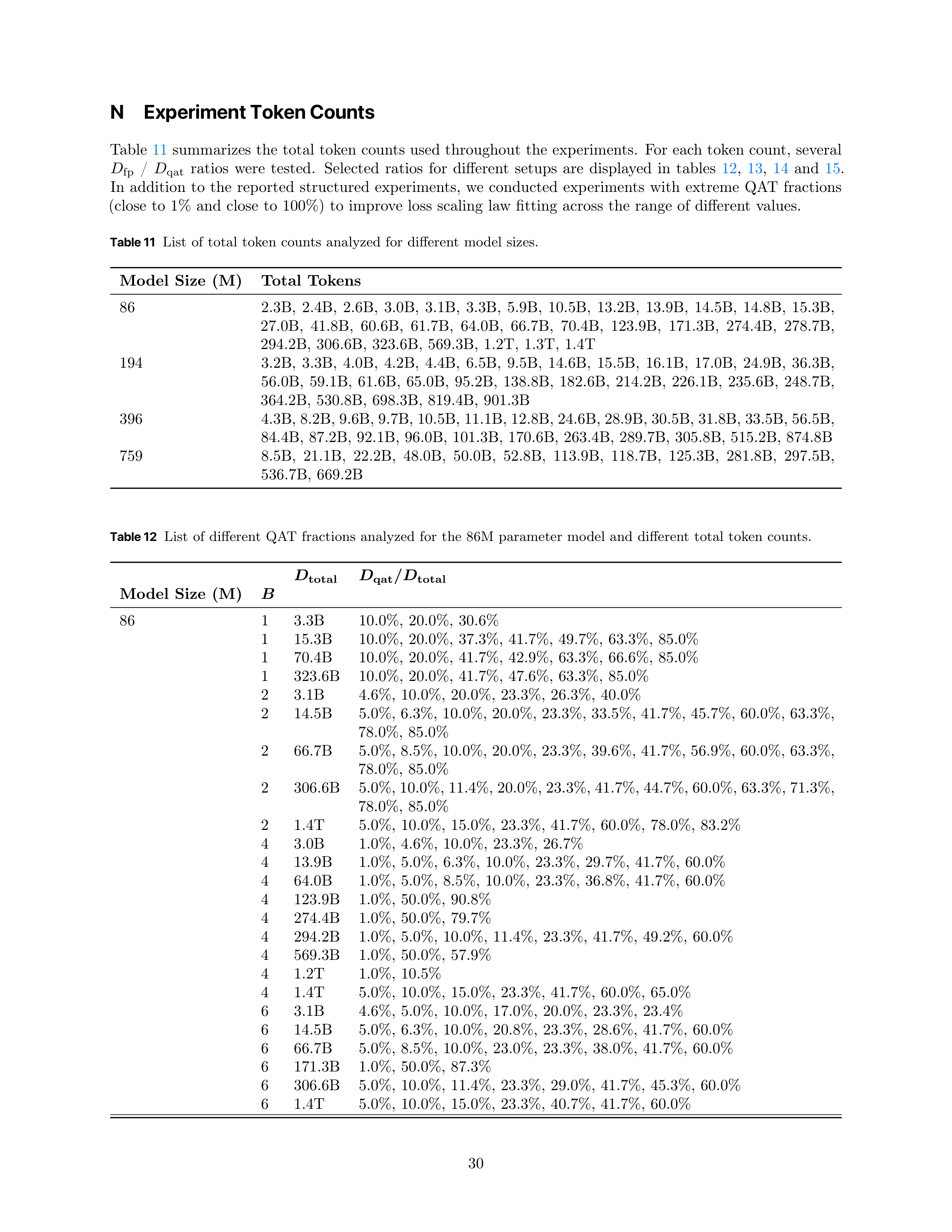
N
Experiment Token Counts
Table
11
summarizes
the
total
token
counts
used
throughout
the
experiments.
For
each
token
count,
several
D
fp
/
D
qat
ratios
were
tested.
Selected
ratios
for
different
setups
are
displayed
in
tables
12
,
13
,
14
and
15
.
In
addition
to
the
reported
structured
experiments,
we
conducted
experiments
with
extreme
QAT
fractions
(close
to
1%
and
close
to
100%)
to
improve
loss
scaling
law
fitting
across
the
range
of
different
values.
Table 11
List
of
total
token
counts
analyzed
for
different
model
sizes.
Model
Size
(M)
Total
Tokens
86
2.3B,
2.4B,
2.6B,
3.0B,
3.1B,
3.3B,
5.9B,
10.5B,
13.2B,
13.9B,
14.5B,
14.8B,
15.3B,
27.0B,
41.8B,
60.6B,
61.7B,
64.0B,
66.7B,
70.4B,
123.9B,
171.3B,
274.4B,
278.7B,
294.2B,
306.6B,
323.6B,
569.3B,
1.2T,
1.3T,
1.4T
194
3.2B,
3.3B,
4.0B,
4.2B,
4.4B,
6.5B,
9.5B,
14.6B,
15.5B,
16.1B,
17.0B,
24.9B,
36.3B,
56.0B,
59.1B,
61.6B,
65.0B,
95.2B,
138.8B,
182.6B,
214.2B,
226.1B,
235.6B,
248.7B,
364.2B,
530.8B,
698.3B,
819.4B,
901.3B
396
4.3B, 8.2B, 9.6B, 9.7B, 10.5B, 11.1B, 12.8B, 24.6B, 28.9B, 30.5B, 31.8B, 33.5B, 56.5B,
84.4B,
87.2B,
92.1B,
96.0B,
101.3B,
170.6B,
263.4B,
289.7B,
305.8B,
515.2B,
874.8B
759
8.5B,
21.1B,
22.2B,
48.0B,
50.0B,
52.8B,
113.9B,
118.7B,
125.3B,
281.8B,
297.5B,
536.7B,
669.2B
Table 12
List
of
different
QAT
fractions
analyzed
for
the
86M
parameter
model
and
different
total
token
counts.
D
total
D
qat
/D
total
Model
Size
(M)
B
86
1
3.3B
10.0%,
20.0%,
30.6%
1
15.3B
10.0%,
20.0%,
37.3%,
41.7%,
49.7%,
63.3%,
85.0%
1
70.4B
10.0%,
20.0%,
41.7%,
42.9%,
63.3%,
66.6%,
85.0%
1
323.6B
10.0%,
20.0%,
41.7%,
47.6%,
63.3%,
85.0%
2
3.1B
4.6%,
10.0%,
20.0%,
23.3%,
26.3%,
40.0%
2
14.5B
5.0%,
6.3%,
10.0%,
20.0%,
23.3%,
33.5%,
41.7%,
45.7%,
60.0%,
63.3%,
78.0%,
85.0%
2
66.7B
5.0%,
8.5%,
10.0%,
20.0%,
23.3%,
39.6%,
41.7%,
56.9%,
60.0%,
63.3%,
78.0%,
85.0%
2
306.6B
5.0%, 10.0%, 11.4%, 20.0%, 23.3%, 41.7%, 44.7%, 60.0%, 63.3%, 71.3%,
78.0%,
85.0%
2
1.4T
5.0%,
10.0%,
15.0%,
23.3%,
41.7%,
60.0%,
78.0%,
83.2%
4
3.0B
1.0%,
4.6%,
10.0%,
23.3%,
26.7%
4
13.9B
1.0%,
5.0%,
6.3%,
10.0%,
23.3%,
29.7%,
41.7%,
60.0%
4
64.0B
1.0%,
5.0%,
8.5%,
10.0%,
23.3%,
36.8%,
41.7%,
60.0%
4
123.9B
1.0%,
50.0%,
90.8%
4
274.4B
1.0%,
50.0%,
79.7%
4
294.2B
1.0%,
5.0%,
10.0%,
11.4%,
23.3%,
41.7%,
49.2%,
60.0%
4
569.3B
1.0%,
50.0%,
57.9%
4
1.2T
1.0%,
10.5%
4
1.4T
5.0%,
10.0%,
15.0%,
23.3%,
41.7%,
60.0%,
65.0%
6
3.1B
4.6%,
5.0%,
10.0%,
17.0%,
20.0%,
23.3%,
23.4%
6
14.5B
5.0%,
6.3%,
10.0%,
20.8%,
23.3%,
28.6%,
41.7%,
60.0%
6
66.7B
5.0%,
8.5%,
10.0%,
23.0%,
23.3%,
38.0%,
41.7%,
60.0%
6
171.3B
1.0%,
50.0%,
87.3%
6
306.6B
5.0%,
10.0%,
11.4%,
23.3%,
29.0%,
41.7%,
45.3%,
60.0%
6
1.4T
5.0%,
10.0%,
15.0%,
23.3%,
40.7%,
41.7%,
60.0%
30
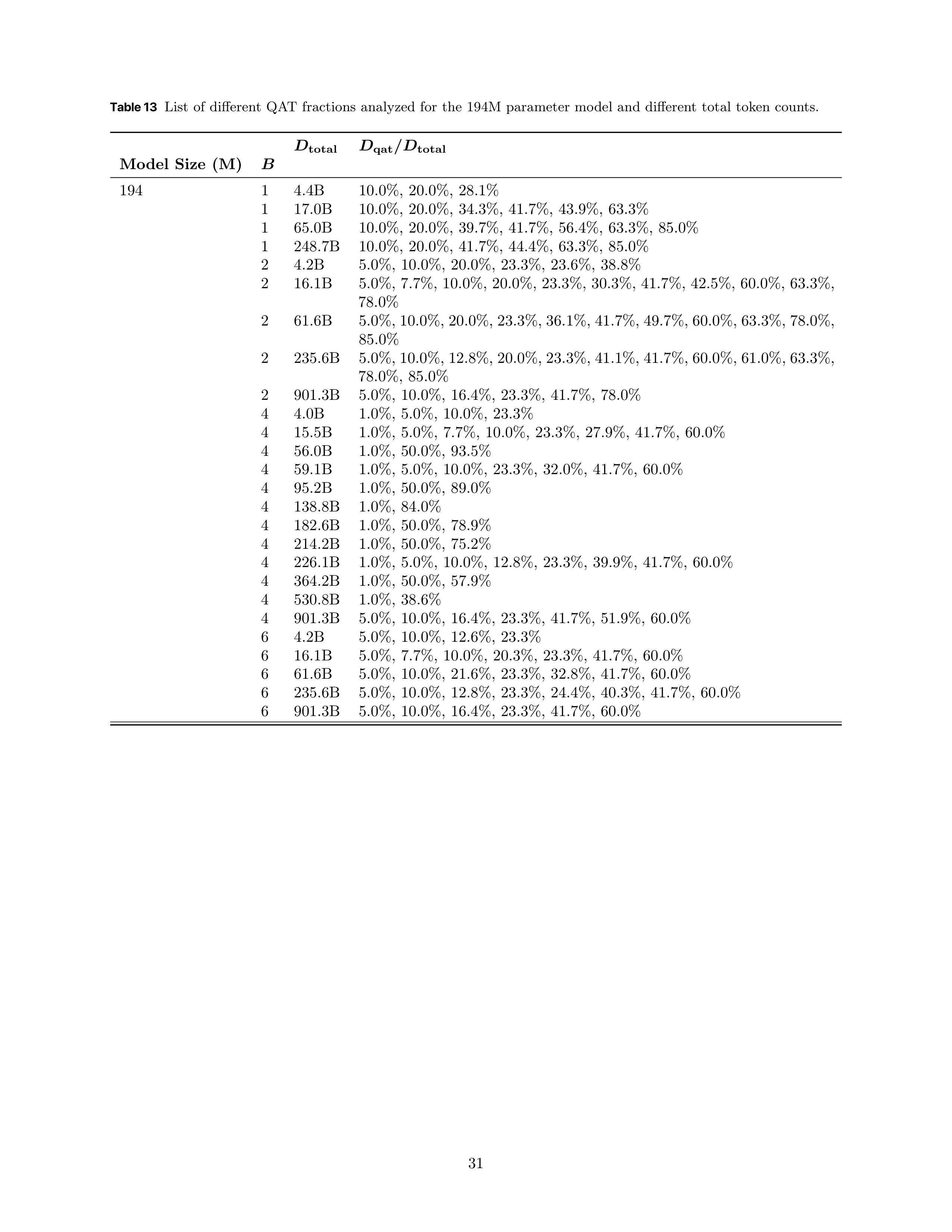
Table 13
List
of
different
QAT
fractions
analyzed
for
the
194M
parameter
model
and
different
total
token
counts.
D
total
D
qat
/D
total
Model
Size
(M)
B
194
1
4.4B
10.0%,
20.0%,
28.1%
1
17.0B
10.0%,
20.0%,
34.3%,
41.7%,
43.9%,
63.3%
1
65.0B
10.0%,
20.0%,
39.7%,
41.7%,
56.4%,
63.3%,
85.0%
1
248.7B
10.0%,
20.0%,
41.7%,
44.4%,
63.3%,
85.0%
2
4.2B
5.0%,
10.0%,
20.0%,
23.3%,
23.6%,
38.8%
2
16.1B
5.0%,
7.7%,
10.0%,
20.0%,
23.3%,
30.3%,
41.7%,
42.5%,
60.0%,
63.3%,
78.0%
2
61.6B
5.0%, 10.0%, 20.0%, 23.3%, 36.1%, 41.7%, 49.7%, 60.0%, 63.3%, 78.0%,
85.0%
2
235.6B
5.0%, 10.0%, 12.8%, 20.0%, 23.3%, 41.1%, 41.7%, 60.0%, 61.0%, 63.3%,
78.0%,
85.0%
2
901.3B
5.0%,
10.0%,
16.4%,
23.3%,
41.7%,
78.0%
4
4.0B
1.0%,
5.0%,
10.0%,
23.3%
4
15.5B
1.0%,
5.0%,
7.7%,
10.0%,
23.3%,
27.9%,
41.7%,
60.0%
4
56.0B
1.0%,
50.0%,
93.5%
4
59.1B
1.0%,
5.0%,
10.0%,
23.3%,
32.0%,
41.7%,
60.0%
4
95.2B
1.0%,
50.0%,
89.0%
4
138.8B
1.0%,
84.0%
4
182.6B
1.0%,
50.0%,
78.9%
4
214.2B
1.0%,
50.0%,
75.2%
4
226.1B
1.0%,
5.0%,
10.0%,
12.8%,
23.3%,
39.9%,
41.7%,
60.0%
4
364.2B
1.0%,
50.0%,
57.9%
4
530.8B
1.0%,
38.6%
4
901.3B
5.0%,
10.0%,
16.4%,
23.3%,
41.7%,
51.9%,
60.0%
6
4.2B
5.0%,
10.0%,
12.6%,
23.3%
6
16.1B
5.0%,
7.7%,
10.0%,
20.3%,
23.3%,
41.7%,
60.0%
6
61.6B
5.0%,
10.0%,
21.6%,
23.3%,
32.8%,
41.7%,
60.0%
6
235.6B
5.0%,
10.0%,
12.8%,
23.3%,
24.4%,
40.3%,
41.7%,
60.0%
6
901.3B
5.0%,
10.0%,
16.4%,
23.3%,
41.7%,
60.0%
31
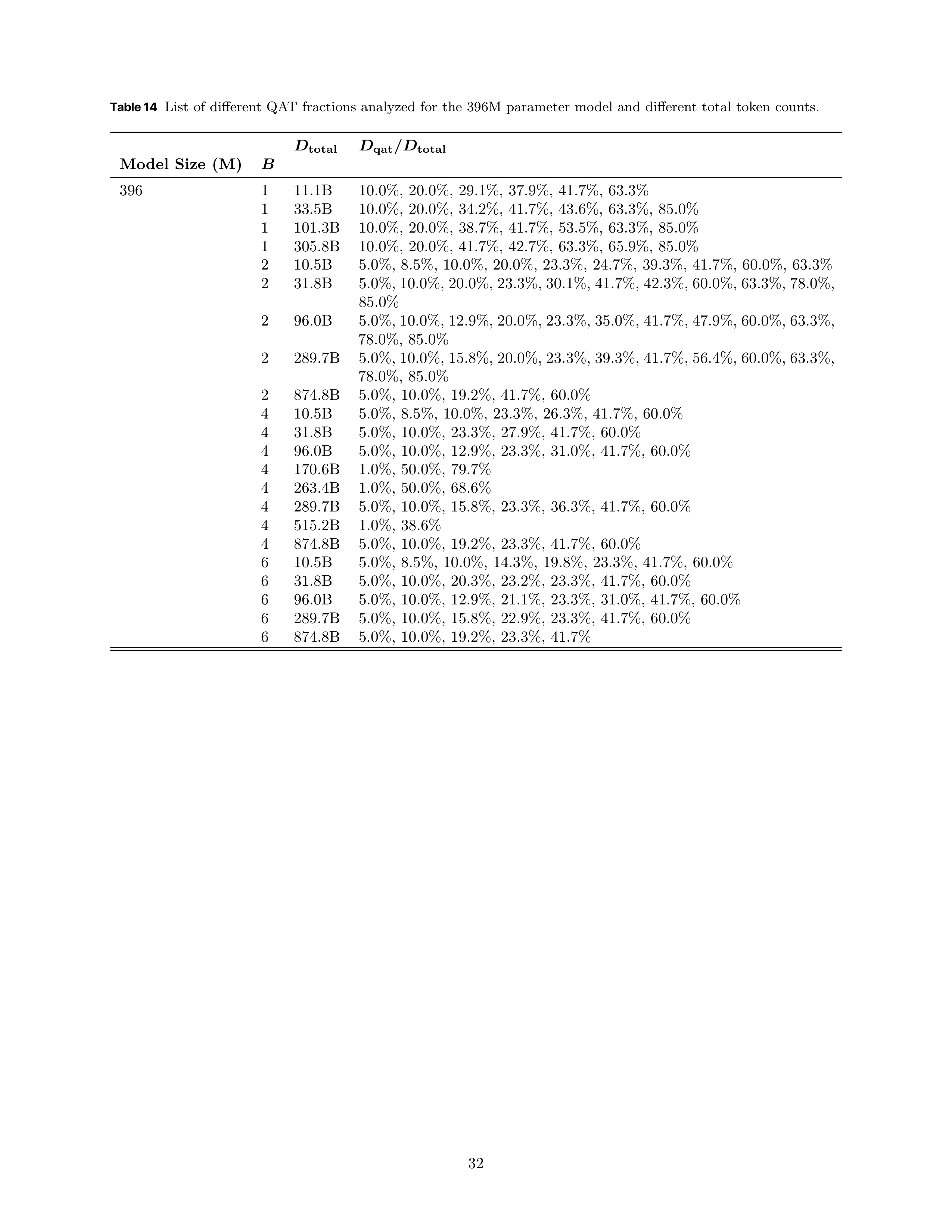
Table 14
List
of
different
QAT
fractions
analyzed
for
the
396M
parameter
model
and
different
total
token
counts.
D
total
D
qat
/D
total
Model
Size
(M)
B
396
1
11.1B
10.0%,
20.0%,
29.1%,
37.9%,
41.7%,
63.3%
1
33.5B
10.0%,
20.0%,
34.2%,
41.7%,
43.6%,
63.3%,
85.0%
1
101.3B
10.0%,
20.0%,
38.7%,
41.7%,
53.5%,
63.3%,
85.0%
1
305.8B
10.0%,
20.0%,
41.7%,
42.7%,
63.3%,
65.9%,
85.0%
2
10.5B
5.0%,
8.5%,
10.0%,
20.0%,
23.3%,
24.7%,
39.3%,
41.7%,
60.0%,
63.3%
2
31.8B
5.0%, 10.0%, 20.0%, 23.3%, 30.1%, 41.7%, 42.3%, 60.0%, 63.3%, 78.0%,
85.0%
2
96.0B
5.0%, 10.0%, 12.9%, 20.0%, 23.3%, 35.0%, 41.7%, 47.9%, 60.0%, 63.3%,
78.0%,
85.0%
2
289.7B
5.0%, 10.0%, 15.8%, 20.0%, 23.3%, 39.3%, 41.7%, 56.4%, 60.0%, 63.3%,
78.0%,
85.0%
2
874.8B
5.0%,
10.0%,
19.2%,
41.7%,
60.0%
4
10.5B
5.0%,
8.5%,
10.0%,
23.3%,
26.3%,
41.7%,
60.0%
4
31.8B
5.0%,
10.0%,
23.3%,
27.9%,
41.7%,
60.0%
4
96.0B
5.0%,
10.0%,
12.9%,
23.3%,
31.0%,
41.7%,
60.0%
4
170.6B
1.0%,
50.0%,
79.7%
4
263.4B
1.0%,
50.0%,
68.6%
4
289.7B
5.0%,
10.0%,
15.8%,
23.3%,
36.3%,
41.7%,
60.0%
4
515.2B
1.0%,
38.6%
4
874.8B
5.0%,
10.0%,
19.2%,
23.3%,
41.7%,
60.0%
6
10.5B
5.0%,
8.5%,
10.0%,
14.3%,
19.8%,
23.3%,
41.7%,
60.0%
6
31.8B
5.0%,
10.0%,
20.3%,
23.2%,
23.3%,
41.7%,
60.0%
6
96.0B
5.0%,
10.0%,
12.9%,
21.1%,
23.3%,
31.0%,
41.7%,
60.0%
6
289.7B
5.0%,
10.0%,
15.8%,
22.9%,
23.3%,
41.7%,
60.0%
6
874.8B
5.0%,
10.0%,
19.2%,
23.3%,
41.7%
32
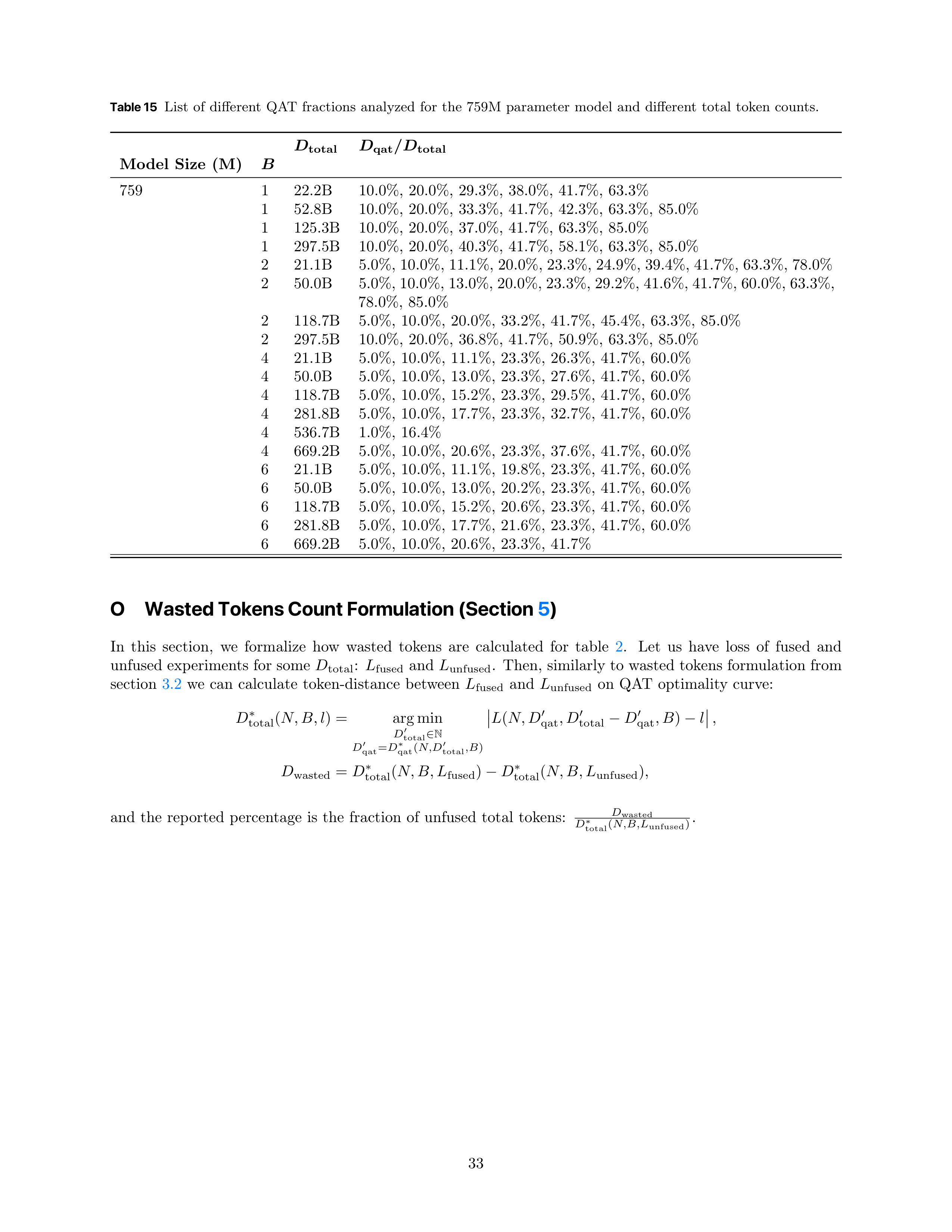
Table 15
List
of
different
QAT
fractions
analyzed
for
the
759M
parameter
model
and
different
total
token
counts.
D
total
D
qat
/D
total
Model
Size
(M)
B
759
1
22.2B
10.0%,
20.0%,
29.3%,
38.0%,
41.7%,
63.3%
1
52.8B
10.0%,
20.0%,
33.3%,
41.7%,
42.3%,
63.3%,
85.0%
1
125.3B
10.0%,
20.0%,
37.0%,
41.7%,
63.3%,
85.0%
1
297.5B
10.0%,
20.0%,
40.3%,
41.7%,
58.1%,
63.3%,
85.0%
2
21.1B
5.0%, 10.0%, 11.1%, 20.0%, 23.3%, 24.9%, 39.4%, 41.7%, 63.3%, 78.0%
2
50.0B
5.0%, 10.0%, 13.0%, 20.0%, 23.3%, 29.2%, 41.6%, 41.7%, 60.0%, 63.3%,
78.0%,
85.0%
2
118.7B
5.0%,
10.0%,
20.0%,
33.2%,
41.7%,
45.4%,
63.3%,
85.0%
2
297.5B
10.0%,
20.0%,
36.8%,
41.7%,
50.9%,
63.3%,
85.0%
4
21.1B
5.0%,
10.0%,
11.1%,
23.3%,
26.3%,
41.7%,
60.0%
4
50.0B
5.0%,
10.0%,
13.0%,
23.3%,
27.6%,
41.7%,
60.0%
4
118.7B
5.0%,
10.0%,
15.2%,
23.3%,
29.5%,
41.7%,
60.0%
4
281.8B
5.0%,
10.0%,
17.7%,
23.3%,
32.7%,
41.7%,
60.0%
4
536.7B
1.0%,
16.4%
4
669.2B
5.0%,
10.0%,
20.6%,
23.3%,
37.6%,
41.7%,
60.0%
6
21.1B
5.0%,
10.0%,
11.1%,
19.8%,
23.3%,
41.7%,
60.0%
6
50.0B
5.0%,
10.0%,
13.0%,
20.2%,
23.3%,
41.7%,
60.0%
6
118.7B
5.0%,
10.0%,
15.2%,
20.6%,
23.3%,
41.7%,
60.0%
6
281.8B
5.0%,
10.0%,
17.7%,
21.6%,
23.3%,
41.7%,
60.0%
6
669.2B
5.0%,
10.0%,
20.6%,
23.3%,
41.7%
O
Wasted Tokens Count Formulation (Section
5
)
In
this
section,
we
formalize
how
wasted
tokens
are
calculated
for
table
2
.
Let
us
have
loss
of
fused
and
unfused
experiments
for
some
D
total
:
L
fused
and
L
unfused
.
Then,
similarly
to
wasted
tokens
formulation
from
section
3.2
we
can
calculate
token-distance
between
L
fused
and
L
unfused
on
QAT
optimality
curve:
D
∗
total
(
N, B, l
) =
arg min
D
′
total
∈
N
D
′
qat
=
D
∗
qat
(
N,D
′
total
,B
)
L
(
N, D
′
qat
, D
′
total
−
D
′
qat
, B
)
−
l
,
D
wasted
=
D
∗
total
(
N, B, L
fused
)
−
D
∗
total
(
N, B, L
unfused
)
,
and
the
reported
percentage
is
the
fraction
of
unfused
total
tokens:
D
wasted
D
∗
total
(
N,B,L
unfused
)
.
33
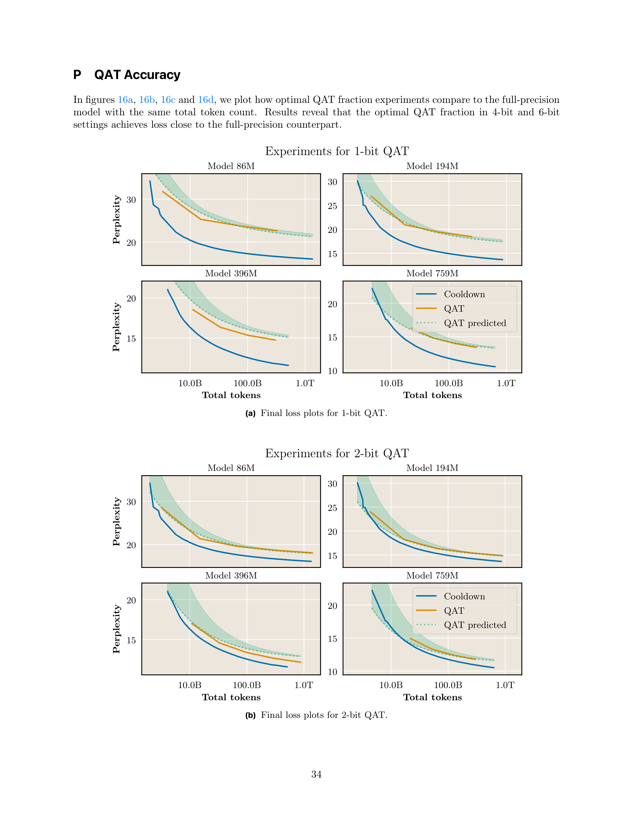
P
QAT Accuracy
In figures
16a
,
16b
,
16c
and
16d
, we plot how optimal QAT fraction experiments compare to the full-precision
model
with
the
same
total
token
count.
Results
reveal
that
the
optimal
QAT
fraction
in
4-bit
and
6-bit
settings
achieves
loss
close
to
the
full-precision
counterpart.
20
30
Perplexity
Model
86M
15
20
25
30
Model
194M
10.0B
100.0B
1.0T
Total
tokens
15
20
Perplexity
Model
396M
10.0B
100.0B
1.0T
Total
tokens
10
15
20
Model
759M
Cooldown
QAT
QAT
predicted
Experiments
for
1-bit
QAT
(a)
Final
loss
plots
for
1-bit
QAT.
20
30
Perplexity
Model
86M
15
20
25
30
Model
194M
10.0B
100.0B
1.0T
Total
tokens
15
20
Perplexity
Model
396M
10.0B
100.0B
1.0T
Total
tokens
10
15
20
Model
759M
Cooldown
QAT
QAT
predicted
Experiments
for
2-bit
QAT
(b)
Final
loss
plots
for
2-bit
QAT.
34
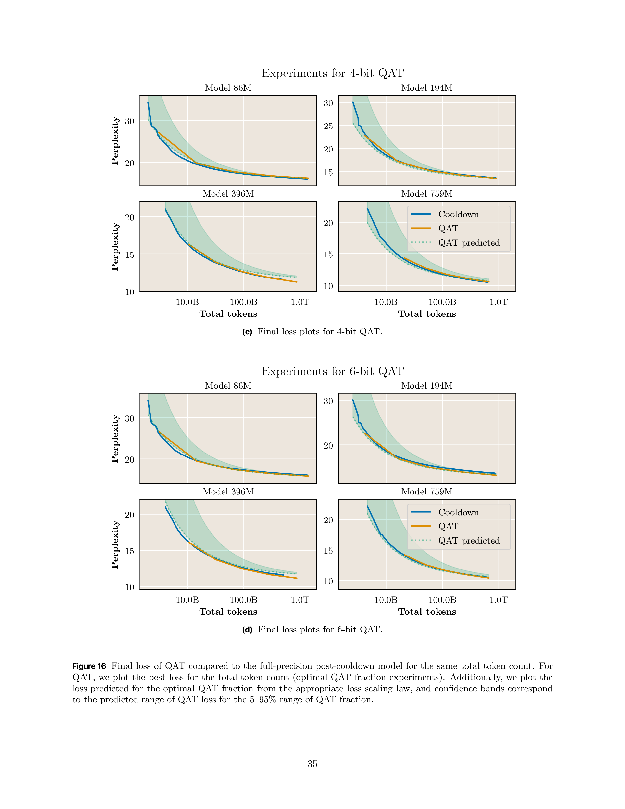
20
30
Perplexity
Model
86M
15
20
25
30
Model
194M
10.0B
100.0B
1.0T
Total
tokens
10
15
20
Perplexity
Model
396M
10.0B
100.0B
1.0T
Total
tokens
10
15
20
Model
759M
Cooldown
QAT
QAT
predicted
Experiments
for
4-bit
QAT
(c)
Final
loss
plots
for
4-bit
QAT.
20
30
Perplexity
Model
86M
20
30
Model
194M
10.0B
100.0B
1.0T
Total
tokens
10
15
20
Perplexity
Model
396M
10.0B
100.0B
1.0T
Total
tokens
10
15
20
Model
759M
Cooldown
QAT
QAT
predicted
Experiments
for
6-bit
QAT
(d)
Final
loss
plots
for
6-bit
QAT.
Figure 16
Final
loss
of
QAT
compared
to
the
full-precision
post-cooldown
model
for
the
same
total
token
count.
For
QAT,
we
plot
the
best
loss
for
the
total
token
count
(optimal
QAT
fraction
experiments).
Additionally,
we
plot
the
loss
predicted
for
the
optimal
QAT
fraction
from
the
appropriate
loss
scaling
law,
and
confidence
bands
correspond
to
the
predicted
range
of
QAT
loss
for
the
5–95%
range
of
QAT
fraction.
35
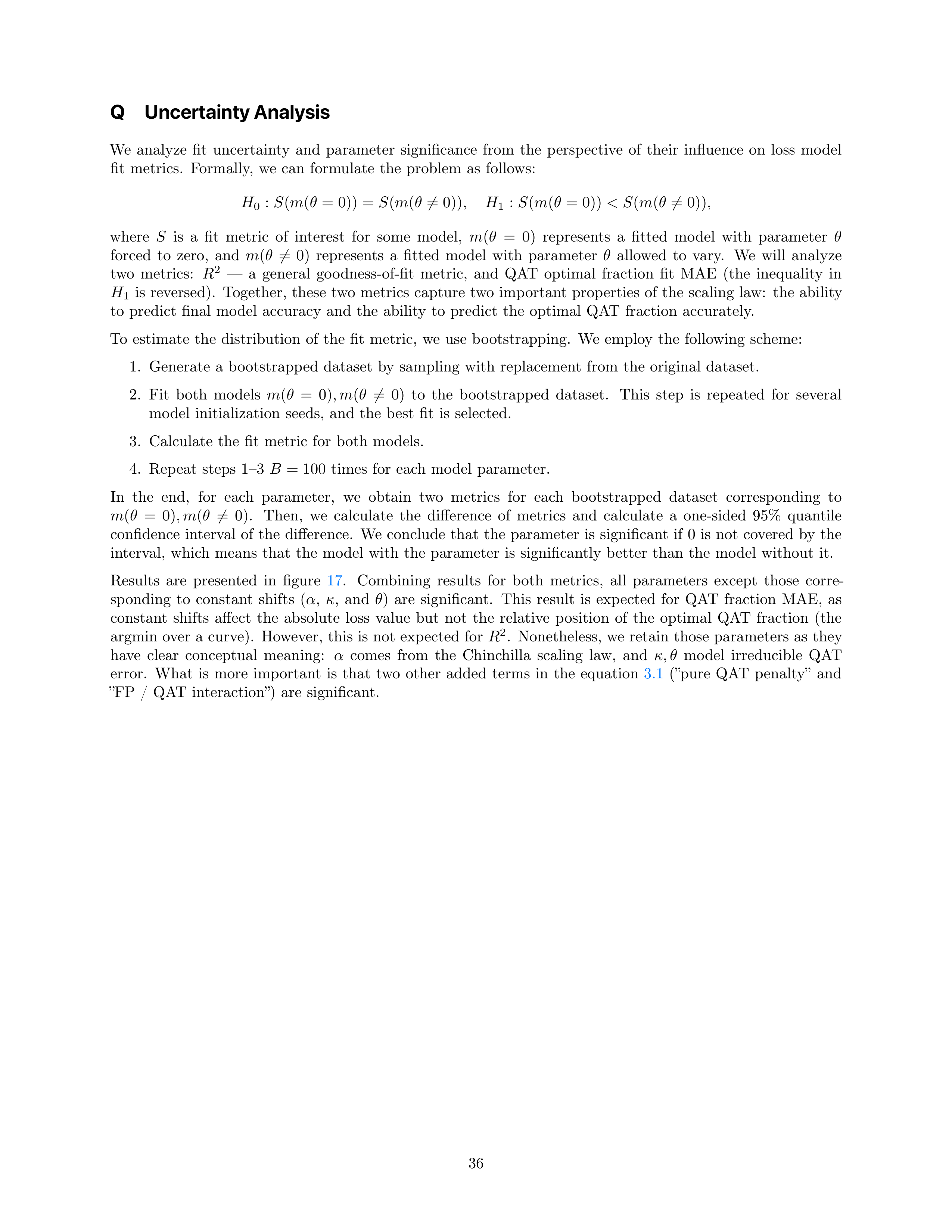
Q
Uncertainty Analysis
We
analyze
fit
uncertainty
and
parameter
significance
from
the
perspective
of
their
influence
on
loss
model
fit
metrics.
Formally,
we
can
formulate
the
problem
as
follows:
H
0
:
S
(
m
(
θ
= 0)) =
S
(
m
(
θ
̸
= 0))
,
H
1
:
S
(
m
(
θ
= 0))
< S
(
m
(
θ
̸
= 0))
,
where
S
is
a
fit
metric
of
interest
for
some
model,
m
(
θ
=
0)
represents
a
fitted
model
with
parameter
θ
forced
to
zero,
and
m
(
θ
̸
=
0)
represents
a
fitted
model
with
parameter
θ
allowed
to
vary.
We
will
analyze
two
metrics:
R
2
—
a
general
goodness-of-fit
metric,
and
QAT
optimal
fraction
fit
MAE
(the
inequality
in
H
1
is
reversed).
Together,
these
two
metrics
capture
two
important
properties
of
the
scaling
law:
the
ability
to
predict
final
model
accuracy
and
the
ability
to
predict
the
optimal
QAT
fraction
accurately.
To
estimate
the
distribution
of
the
fit
metric,
we
use
bootstrapping.
We
employ
the
following
scheme:
1.
Generate
a
bootstrapped
dataset
by
sampling
with
replacement
from
the
original
dataset.
2.
Fit
both
models
m
(
θ
=
0)
, m
(
θ
̸
=
0)
to
the
bootstrapped
dataset.
This
step
is
repeated
for
several
model
initialization
seeds,
and
the
best
fit
is
selected.
3.
Calculate
the
fit
metric
for
both
models.
4.
Repeat
steps
1–3
B
= 100
times
for
each
model
parameter.
In
the
end,
for
each
parameter,
we
obtain
two
metrics
for
each
bootstrapped
dataset
corresponding
to
m
(
θ
=
0)
, m
(
θ
̸
=
0)
.
Then,
we
calculate
the
difference
of
metrics
and
calculate
a
one-sided
95%
quantile
confidence
interval
of
the
difference.
We
conclude
that
the
parameter
is
significant
if
0
is
not
covered
by
the
interval,
which
means
that
the
model
with
the
parameter
is
significantly
better
than
the
model
without
it.
Results
are
presented
in
figure
17
.
Combining
results
for
both
metrics,
all
parameters
except
those
corre-
sponding
to
constant
shifts
(
α
,
κ
,
and
θ
)
are
significant.
This
result
is
expected
for
QAT
fraction
MAE,
as
constant
shifts
affect
the
absolute
loss
value
but
not
the
relative
position
of
the
optimal
QAT
fraction
(the
argmin
over
a
curve).
However,
this
is
not
expected
for
R
2
.
Nonetheless,
we
retain
those
parameters
as
they
have
clear
conceptual
meaning:
α
comes
from
the
Chinchilla
scaling
law,
and
κ, θ
model
irreducible
QAT
error.
What
is
more
important
is
that
two
other
added
terms
in
the
equation
3.1
(”pure
QAT
penalty”
and
”FP
/
QAT
interaction”)
are
significant.
36
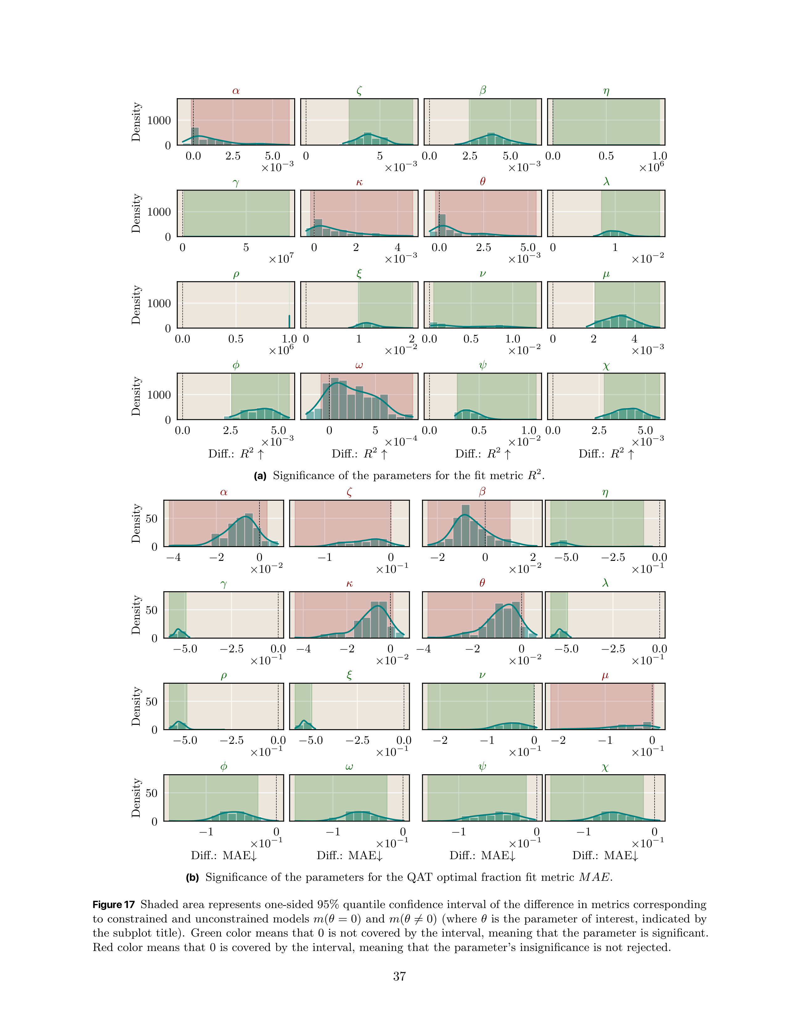
0
.
0
2
.
5
5
.
0
×
10
−
3
0
1000
Density
α
0
5
×
10
−
3
ζ
0
.
0
2
.
5
5
.
0
×
10
−
3
β
0
.
0
0
.
5
1
.
0
×
10
6
η
0
5
×
10
7
0
1000
Density
γ
0
2
4
×
10
−
3
κ
0
.
0
2
.
5
5
.
0
×
10
−
3
θ
0
1
×
10
−
2
λ
0
.
0
0
.
5
1
.
0
×
10
6
0
1000
Density
ρ
0
1
2
×
10
−
2
ξ
0
.
0
0
.
5
1
.
0
×
10
−
2
ν
0
2
4
×
10
−
3
µ
0
.
0
2
.
5
5
.
0
Diff.:
R
2
↑
×
10
−
3
0
1000
Density
ϕ
0
5
Diff.:
R
2
↑
×
10
−
4
ω
0
.
0
0
.
5
1
.
0
Diff.:
R
2
↑
×
10
−
2
ψ
0
.
0
2
.
5
5
.
0
Diff.:
R
2
↑
×
10
−
3
χ
(a)
Significance
of
the
parameters
for
the
fit
metric
R
2
.
−
4
−
2
0
×
10
−
2
0
50
Density
α
−
1
0
×
10
−
1
ζ
−
2
0
2
×
10
−
2
β
−
5
.
0
−
2
.
5
0
.
0
×
10
−
1
η
−
5
.
0
−
2
.
5
0
.
0
×
10
−
1
0
50
Density
γ
−
4
−
2
0
×
10
−
2
κ
−
4
−
2
0
×
10
−
2
θ
−
5
.
0
−
2
.
5
0
.
0
×
10
−
1
λ
−
5
.
0
−
2
.
5
0
.
0
×
10
−
1
0
50
Density
ρ
−
5
.
0
−
2
.
5
0
.
0
×
10
−
1
ξ
−
2
−
1
0
×
10
−
1
ν
−
2
−
1
0
×
10
−
1
µ
−
1
0
Diff.:
MAE
↓
×
10
−
1
0
50
Density
ϕ
−
1
0
Diff.:
MAE
↓
×
10
−
1
ω
−
1
0
Diff.:
MAE
↓
×
10
−
1
ψ
−
1
0
Diff.:
MAE
↓
×
10
−
1
χ
(b)
Significance
of
the
parameters
for
the
QAT
optimal
fraction
fit
metric
MAE
.
Figure 17
Shaded
area
represents
one-sided
95%
quantile
confidence
interval
of
the
difference
in
metrics
corresponding
to
constrained
and
unconstrained
models
m
(
θ
= 0)
and
m
(
θ
̸
= 0)
(where
θ
is
the
parameter
of
interest,
indicated
by
the
subplot
title).
Green
color
means
that
0
is
not
covered
by
the
interval,
meaning
that
the
parameter
is
significant.
Red
color
means
that
0
is
covered
by
the
interval,
meaning
that
the
parameter’s
insignificance
is
not
rejected.
37
R
Future Work
In this section, we speculate on possible results for the future work directions proposed in the paper (section
6
).
R.1
Pretrain Precision & QAT Precision Interaction
The
question
of
interest
is
“How
do
QAT
scaling
laws
change
when
pretrain
precision
is
reduced?”
Specifically,
a
practically
important
question
is
how
optimal
QAT
compute
allocation
changes.
Kumar
et
al.
(
2025
)
analyze
this
question
in
the
context
of
post-training
quantization.
While
QAT
and
PTQ
yield
significant
differences
in
accuracy
(especially
for
lower
bits
(
Liu
et
al.
,
2025
)),
we
expect
general
trends
to
be
similar.
Kumar
et
al.
(
2025
)
report
that
“overall,
models
trained
in
lower
precision
are
more
robust
to
post-training
quantization in the sense of incurring lower degradation.”
We expect the same phenomenon in the context of
QAT. Therefore, one may expect the optimal QAT fraction to be smaller when a model is pretrained in lower
floating-point precisions (fp4, fp8) than in high precision (fp16, bf16, fp32).
Still, we expect the optimal QAT
fraction
to
grow
with
increasing
total
compute.
R.2
QAT Scaling Law for Multi-Stage Pretraining
Current state-of-the-art chat models commonly incorporate multiple training stages.
Commonly, after general
cross-entropy
pretraining,
additional
supervised
fine-tuning
(SFT)
and
reinforcement
learning
stages
are
performed
(
DeepSeek-AI
et
al.
,
2025
;
OLMo
et
al.
,
2025
;
Apertus
et
al.
,
2025
;
Ouyang
et
al.
,
2022
;
Allal
et al.
,
2025
;
Rafailov et al.
,
2023
;
Schulman et al.
,
2017
;
Zhou et al.
,
2025a
).
This raises not only the question
of
how
much
compute
to
allocate
for
QAT
but
also
how
to
distribute
this
compute
among
different
stages.
A
possible
solution
is
to
conduct
all
post-pretraining
stages
over
the
QAT
model.
Usually,
post-training
constitutes
a
minor
percentage
of
compute
when
compared
to
pretraining
(
DeepSeek-AI
et
al.
,
2025
;
Allal
et
al.
,
2025
;
OLMo
et
al.
,
2025
;
Apertus
et
al.
,
2025
).
Therefore,
it
is
natural
to
expect
the
optimal
QAT
fraction
to
be
larger
than
the
entire
post-pretraining
stage.
This
means
that
it
is
possible
to
start
QAT
during
pretraining
and
finish
QAT
with
post-pretraining
tuning.
Such
a
methodology
is
also
motivated
by
the
fact
that
QAT
incurs
representation
changes,
especially
in
the
case
of
small
QAT
bit-widths
(
Liu
et
al.
,
2025
).
Therefore,
we
believe
it
is
beneficial
not
to
postpone
this
process
of
representation
change
until
after
post-pretraining
stages.
Apple and the Apple logo are trademarks of Apple Inc., registered in the U.S. and other countries and regions.
38