XGBoost:
A Scalable Tree Boosting System
Tianqi Chen
University of Washington
tqchen@cs.washington.edu
Carlos Guestrin
University of Washington
guestrin@cs.washington.edu
ABSTRACT
Tree
boosting
is
a
highly
effective
and
widely
used
machine
learning
method.
In
this
paper,
we
describe
a
scalable
end-
to-end
tree
boosting
system
called
XGBoost,
which
is
used
widely
by
data
scientists
to
achieve
state-of-the-art
results
on
many
machine
learning
challenges.
We
propose
a
novel
sparsity-aware algorithm for sparse data and weighted quan-
tile sketch for approximate tree learning.
More importantly,
we
provide
insights
on
cache
access
patterns,
data
compres-
sion
and
sharding
to
build
a
scalable
tree
boosting
system.
By combining these insights, XGBoost scales beyond billions
of examples using far fewer resources than existing systems.
Keywords
Large-scale
Machine
Learning
1.
INTRODUCTION
Machine
learning
and
data-driven
approaches
are
becom-
ing
very
important
in
many
areas.
Smart
spam
classifiers
protect our email by learning from massive amounts of spam
data
and
user
feedback;
advertising
systems
learn
to
match
the right ads with the right context; fraud detection systems
protect
banks
from
malicious
attackers;
anomaly
event
de-
tection
systems
help
experimental
physicists
to
find
events
that
lead
to
new
physics.
There
are
two
important
factors
that
drive
these
successful
applications:
usage
of
effective
(statistical)
models
that
capture
the
complex
data
depen-
dencies
and
scalable
learning
systems
that
learn
the
model
of
interest
from
large
datasets.
Among
the
machine
learning
methods
used
in
practice,
gradient
tree
boosting
[
10
]
1
is
one
technique
that
shines
in
many
applications.
Tree
boosting
has
been
shown
to
give
state-of-the-art
results
on
many
standard
classification
benchmarks [
16
].
LambdaMART [
5
], a variant of tree boost-
ing
for
ranking,
achieves
state-of-the-art
result
for
ranking
1
Gradient
tree
boosting
is
also
known
as
gradient
boosting
machine (GBM) or gradient boosted regression tree (GBRT)
Permission
to
make
digital
or
hard
copies
of
part
or
all
of
this
work
for
personal
or
classroom use is granted without fee provided that copies are not made or distributed
for profit or commercial advantage and that copies bear this notice and the full citation
on the first page. Copyrights for third-party components of this work must be honored.
For all other uses, contact the owner/author(s).
KDD ’16, August 13-17, 2016, San Francisco, CA, USA
c
⃝
2016 Copyright held by the owner/author(s).
ACM ISBN .
DOI:
problems.
Besides
being
used
as
a
stand-alone
predictor,
it
is
also
incorporated
into
real-world
production
pipelines
for
ad
click
through
rate
prediction
[
15
].
Finally,
it
is
the
de-
facto
choice
of
ensemble
method
and
is
used
in
challenges
such
as
the
Netflix
prize
[
3
].
In
this
paper,
we
describe
XGBoost,
a
scalable
machine
learning system for tree boosting.
The system is available as
an open source package
2
.
The impact of the system has been
widely recognized in a number of machine learning and data
mining
challenges.
Take
the
challenges
hosted
by
the
ma-
chine
learning
competition
site
Kaggle
for
example.
Among
the
29
challenge
winning
solutions
3
published
at
Kaggle’s
blog
during
2015,
17
solutions
used
XGBoost.
Among
these
solutions,
eight
solely
used
XGBoost
to
train
the
model,
while most others combined XGBoost with neural nets in en-
sembles.
For
comparison,
the
second
most
popular
method,
deep
neural
nets,
was
used
in
11
solutions.
The
success
of
the
system
was
also
witnessed
in
KDDCup
2015,
where
XGBoost
was
used
by
every
winning
team
in
the
top-10.
Moreover,
the
winning
teams
reported
that
ensemble
meth-
ods
outperform
a
well-configured
XGBoost
by
only
a
small
amount
[
1
].
These
results
demonstrate
that
our
system
gives
state-of-
the-art
results
on
a
wide
range
of
problems.
Examples
of
the
problems
in
these
winning
solutions
include:
store
sales
prediction; high energy physics event classification; web text
classification;
customer
behavior
prediction;
motion
detec-
tion; ad click through rate prediction; malware classification;
product
categorization;
hazard
risk
prediction;
massive
on-
line
course
dropout
rate
prediction.
While
domain
depen-
dent data analysis and feature engineering play an important
role
in
these
solutions,
the
fact
that
XGBoost
is
the
consen-
sus
choice
of
learner
shows
the
impact
and
importance
of
our
system
and
tree
boosting.
The most important factor behind the success of XGBoost
is its scalability in all scenarios.
The system runs more than
ten
times
faster
than
existing
popular
solutions
on
a
single
machine
and
scales
to
billions
of
examples
in
distributed
or
memory-limited
settings.
The
scalability
of
XGBoost
is
due
to several important systems and algorithmic optimizations.
These
innovations
include:
a
novel
tree
learning
algorithm
is for handling
sparse
data
; a theoretically justified weighted
quantile sketch procedure enables handling instance weights
in
approximate
tree
learning.
Parallel
and
distributed
com-
puting makes learning faster which enables quicker model ex-
ploration.
More
importantly,
XGBoost
exploits
out-of-core
2
https://github.com/dmlc/xgboost
3
Solutions
come
from
of
top-3
teams
of
each
competitions.
arXiv:1603.02754v3 [cs.LG] 10 Jun 2016
computation
and
enables
data
scientists
to
process
hundred
millions
of
examples
on
a
desktop.
Finally,
it
is
even
more
exciting
to
combine
these
techniques
to
make
an
end-to-end
system that scales to even larger data with the least amount
of
cluster
resources.
The
major
contributions
of
this
paper
is
listed
as
follows:
•
We
design
and
build
a
highly
scalable
end-to-end
tree
boosting
system.
•
We
propose
a
theoretically
justified
weighted
quantile
sketch
for
efficient
proposal
calculation.
•
We introduce a novel sparsity-aware algorithm for par-
allel
tree
learning.
•
We
propose
an
effective
cache-aware
block
structure
for
out-of-core
tree
learning.
While there are some existing works on parallel tree boost-
ing
[
22
,
23
,
19
],
the
directions
such
as
out-of-core
compu-
tation,
cache-aware
and
sparsity-aware
learning
have
not
been
explored.
More
importantly,
an
end-to-end
system
that
combines
all
of
these
aspects
gives
a
novel
solution
for
real-world
use-cases.
This
enables
data
scientists
as
well
as
researchers
to
build
powerful
variants
of
tree
boosting
al-
gorithms
[
7
,
8
].
Besides
these
major
contributions,
we
also
make
additional
improvements
in
proposing
a
regularized
learning
objective,
which
we
will
include
for
completeness.
The
remainder
of
the
paper
is
organized
as
follows.
We
will
first
review
tree
boosting
and
introduce
a
regularized
objective in Sec.
2
.
We then describe the split finding meth-
ods in Sec.
3
as well as the system design in Sec.
4
, including
experimental
results
when
relevant
to
provide
quantitative
support
for
each
optimization
we
describe.
Related
work
is
discussed
in
Sec.
5
.
Detailed
end-to-end
evaluations
are
included
in
Sec.
6
.
Finally
we
conclude
the
paper
in
Sec.
7
.
2.
TREE BOOSTING IN A NUTSHELL
We
review
gradient
tree
boosting
algorithms
in
this
sec-
tion.
The
derivation
follows
from
the
same
idea
in
existing
literatures in gradient boosting.
Specicially the second order
method is originated from Friedman et al. [
12
].
We make mi-
nor
improvements
in
the
reguralized
objective,
which
were
found
helpful
in
practice.
2.1
Regularized Learning Objective
For
a
given
data
set
with
n
examples
and
m
features
D
=
{
(
x
i
, y
i
)
}
(
|D|
=
n,
x
i
∈
R
m
, y
i
∈
R
),
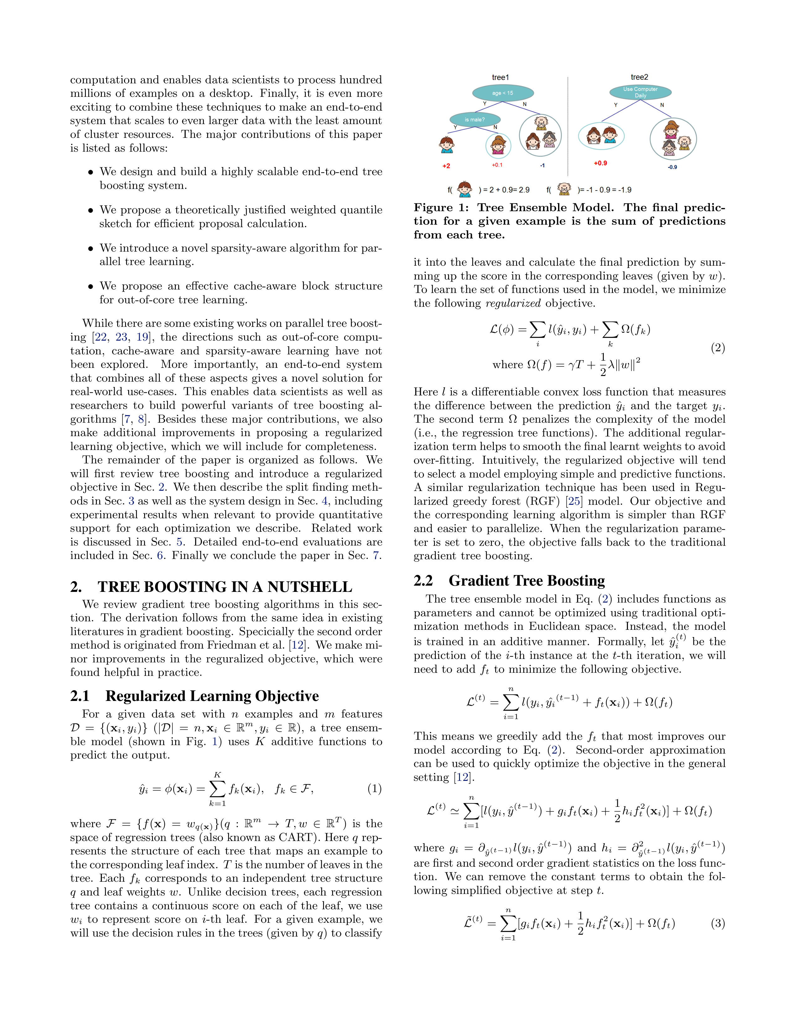
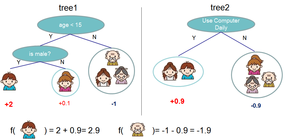
a
tree
ensem-
ble
model
(shown
in
Fig.
1
)
uses
K
additive
functions
to
predict
the
output.
ˆ
y
i
=
φ
(
x
i
) =
K
X
k
=1
f
k
(
x
i
)
,
f
k
∈F
,
(1)
where
F
=
{
f
(
x
)
=
w
q
(
x
)
}
(
q
:
R
m
→
T, w
∈
R
T
)
is
the
space of
regression trees
(also
known
as
CART).
Here
q
rep-
resents
the
structure
of
each
tree
that
maps
an
example
to
the corresponding leaf index.
T
is the number of leaves in the
tree.
Each
f
k
corresponds
to
an
independent
tree
structure
q
and
leaf
weights
w
.
Unlike
decision
trees,
each
regression
tree
contains
a
continuous
score
on
each
of
the
leaf,
we
use
w
i
to
represent
score
on
i
-th
leaf.
For
a
given
example,
we
will use the decision rules in the trees (given by
q
) to classify
Figure
1:
Tree
Ensemble
Model.
The
final
predic-
tion
for
a
given
example
is
the
sum
of
predictions
from
each
tree.
it
into
the
leaves
and
calculate
the
final
prediction
by
sum-
ming
up
the
score
in
the
corresponding
leaves
(given
by
w
).
To learn the set of functions used in the model, we minimize
the
following
regularized
objective.
L
(
φ
) =
X
i
l
(ˆ
y
i
, y
i
) +
X
k
Ω(
f
k
)
where
Ω(
f
) =
γT
+
1
2
λ
∥
w
∥
2
(2)
Here
l
is
a
differentiable
convex
loss
function
that
measures
the
difference
between
the
prediction
ˆ
y
i
and
the
target
y
i
.
The
second
term
Ωpenalizes
the
complexity
of
the
model
(i.e.,
the
regression
tree
functions).
The
additional
regular-
ization term helps to smooth the final learnt weights to avoid
over-fitting.
Intuitively,
the
regularized
objective
will
tend
to select a model employing simple and predictive functions.
A
similar
regularization
technique
has
been
used
in
Regu-
larized
greedy
forest
(RGF)
[
25
]
model.
Our
objective
and
the
corresponding
learning
algorithm
is
simpler
than
RGF
and
easier
to
parallelize.
When
the
regularization
parame-
ter
is
set
to
zero,
the
objective
falls
back
to
the
traditional
gradient
tree
boosting.
2.2
Gradient Tree Boosting
The
tree
ensemble
model
in
Eq.
(
2
)
includes
functions
as
parameters
and
cannot
be
optimized
using
traditional
opti-
mization
methods
in
Euclidean
space.
Instead,
the
model
is
trained
in
an
additive
manner.
Formally,
let
ˆ
y
(
t
)
i
be
the
prediction
of
the
i
-th
instance
at
the
t
-th
iteration,
we
will
need
to
add
f
t
to
minimize
the
following
objective.
L
(
t
)
=
n
X
i
=1
l
(
y
i
,
ˆ
y
i
(
t
−
1)
+
f
t
(
x
i
)) + Ω(
f
t
)
This
means
we
greedily
add
the
f
t
that
most
improves
our
model
according
to
Eq.
(
2
).
Second-order
approximation
can
be
used
to
quickly
optimize
the
objective
in
the
general
setting
[
12
].
L
(
t
)
≃
n
X
i
=1
[
l
(
y
i
,
ˆ
y
(
t
−
1)
) +
g
i
f
t
(
x
i
) +
1
2
h
i
f
2
t
(
x
i
)] + Ω(
f
t
)
where
g
i
=
∂
ˆ
y
(
t
−
1)
l
(
y
i
,
ˆ
y
(
t
−
1)
)
and
h
i
=
∂
2
ˆ
y
(
t
−
1)
l
(
y
i
,
ˆ
y
(
t
−
1)
)
are first and second order gradient statistics on the loss func-
tion.
We
can
remove
the
constant
terms
to
obtain
the
fol-
lowing
simplified
objective
at
step
t
.
˜
L
(
t
)
=
n
X
i
=1
[
g
i
f
t
(
x
i
) +
1
2
h
i
f
2
t
(
x
i
)] + Ω(
f
t
)
(3)
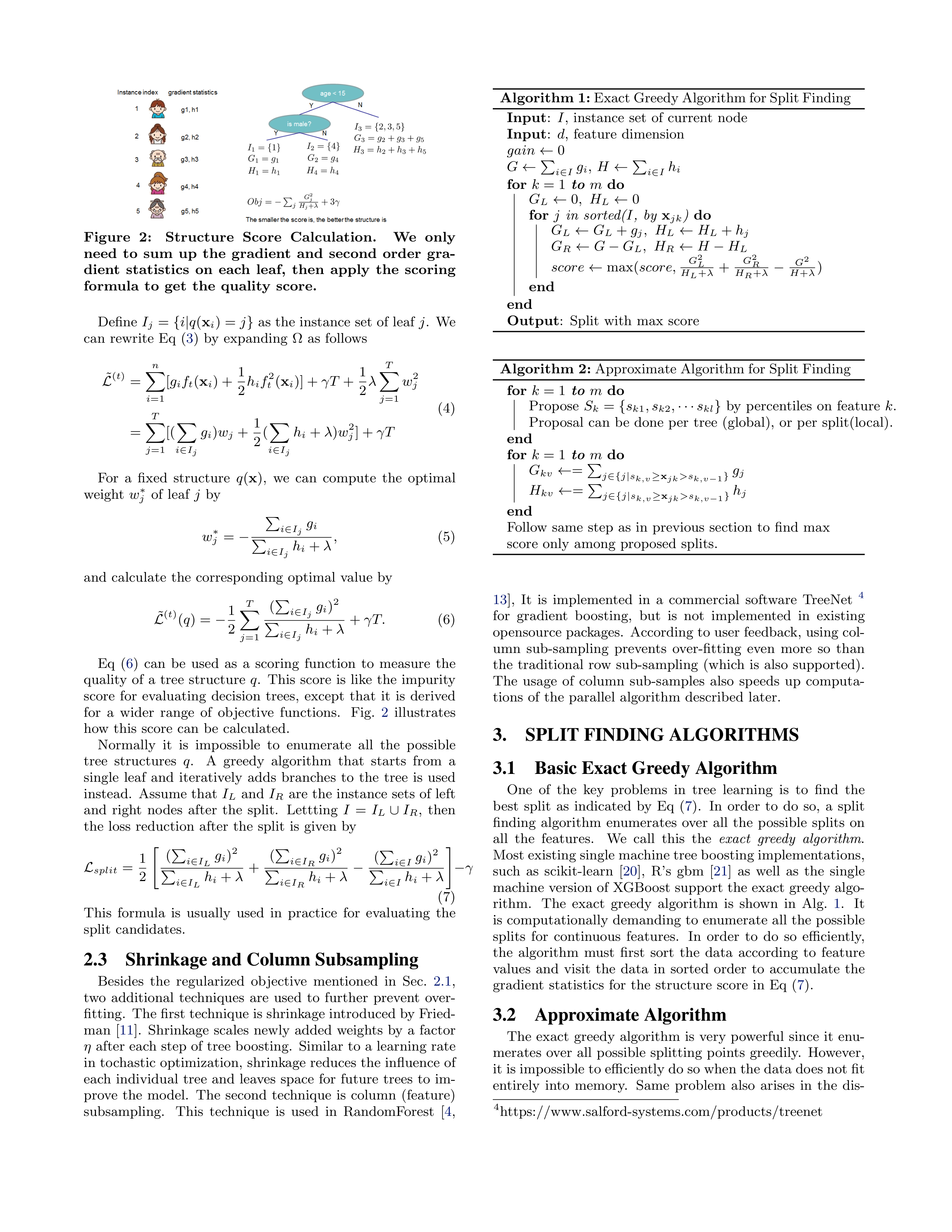
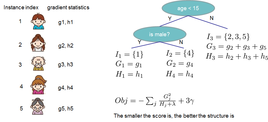
Figure
2:
Structure
Score
Calculation.
We
only
need
to
sum
up
the
gradient
and
second
order
gra-
dient
statistics
on
each
leaf,
then
apply
the
scoring
formula
to
get
the
quality
score.
Define
I
j
=
{
i
|
q
(
x
i
) =
j
}
as
the
instance
set
of
leaf
j
.
We
can
rewrite
Eq
(
3
)
by
expanding
Ωas
follows
˜
L
(
t
)
=
n
X
i
=1
[
g
i
f
t
(
x
i
) +
1
2
h
i
f
2
t
(
x
i
)] +
γT
+
1
2
λ
T
X
j
=1
w
2
j
=
T
X
j
=1
[(
X
i
∈
I
j
g
i
)
w
j
+
1
2
(
X
i
∈
I
j
h
i
+
λ
)
w
2
j
] +
γT
(4)
For
a
fixed
structure
q
(
x
),
we
can
compute
the
optimal
weight
w
∗
j
of
leaf
j
by
w
∗
j
=
−
P
i
∈
I
j
g
i
P
i
∈
I
j
h
i
+
λ,
(5)
and
calculate
the
corresponding
optimal
value
by
˜
L
(
t
)
(
q
) =
−
1
2
T
X
j
=1
(
P
i
∈
I
j
g
i
)
2
P
i
∈
I
j
h
i
+
λ
+
γT.
(6)
Eq
(
6
)
can
be
used
as
a
scoring
function
to
measure
the
quality
of
a
tree
structure
q
.
This
score
is
like
the
impurity
score
for
evaluating
decision
trees,
except
that
it
is
derived
for
a
wider
range
of
objective
functions.
Fig.
2
illustrates
how
this
score
can
be
calculated.
Normally
it
is
impossible
to
enumerate
all
the
possible
tree
structures
q
.
A
greedy
algorithm
that
starts
from
a
single
leaf
and
iteratively
adds
branches
to
the
tree
is
used
instead.
Assume
that
I
L
and
I
R
are
the
instance
sets
of
left
and
right
nodes
after
the
split.
Lettting
I
=
I
L
∪
I
R
,
then
the
loss
reduction
after
the
split
is
given
by
L
split
=
1
2
"
(
P
i
∈
I
L
g
i
)
2
P
i
∈
I
L
h
i
+
λ
+
(
P
i
∈
I
R
g
i
)
2
P
i
∈
I
R
h
i
+
λ
−
(
P
i
∈
I
g
i
)
2
P
i
∈
I
h
i
+
λ
#
−
γ
(7)
This
formula
is
usually
used
in
practice
for
evaluating
the
split
candidates.
2.3
Shrinkage and Column Subsampling
Besides
the
regularized
objective
mentioned
in
Sec.
2.1
,
two
additional
techniques
are
used
to
further
prevent
over-
fitting.
The first technique is shrinkage introduced by Fried-
man
[
11
].
Shrinkage
scales
newly
added
weights
by
a
factor
η
after
each
step
of
tree
boosting.
Similar
to
a
learning
rate
in
tochastic
optimization,
shrinkage
reduces
the
influence
of
each
individual
tree
and
leaves
space
for
future
trees
to
im-
prove
the
model.
The
second
technique
is
column
(feature)
subsampling.
This
technique
is
used
in
RandomForest
[
4
,
Algorithm 1:
Exact Greedy Algorithm for Split Finding
Input
:
I
,
instance
set
of
current
node
Input
:
d
,
feature
dimension
gain
←
0
G
←
P
i
∈
I
g
i
,
H
←
P
i
∈
I
h
i
for
k
= 1
to
m
do
G
L
←
0
,
H
L
←
0
for
j
in
sorted(
I
,
by
x
jk
)
do
G
L
←
G
L
+
g
j
,
H
L
←
H
L
+
h
j
G
R
←
G
−
G
L
,
H
R
←
H
−
H
L
score
←
max(
score,
G
2
L
H
L
+
λ
+
G
2
R
H
R
+
λ
−
G
2
H
+
λ
)
end
end
Output
:
Split
with
max
score
Algorithm
2:
Approximate Algorithm for Split Finding
for
k
= 1
to
m
do
Propose
S
k
=
{
s
k
1
, s
k
2
,
· · ·
s
kl
}
by
percentiles
on
feature
k
.
Proposal
can
be
done
per
tree
(global),
or
per
split(local).
end
for
k
= 1
to
m
do
G
kv
←
=
P
j
∈{
j
|
s
k,v
≥
x
jk
>s
k,v
−
1
}
g
j
H
kv
←
=
P
j
∈{
j
|
s
k,v
≥
x
jk
>s
k,v
−
1
}
h
j
end
Follow
same
step
as
in
previous
section
to
find
max
score
only
among
proposed
splits.
13
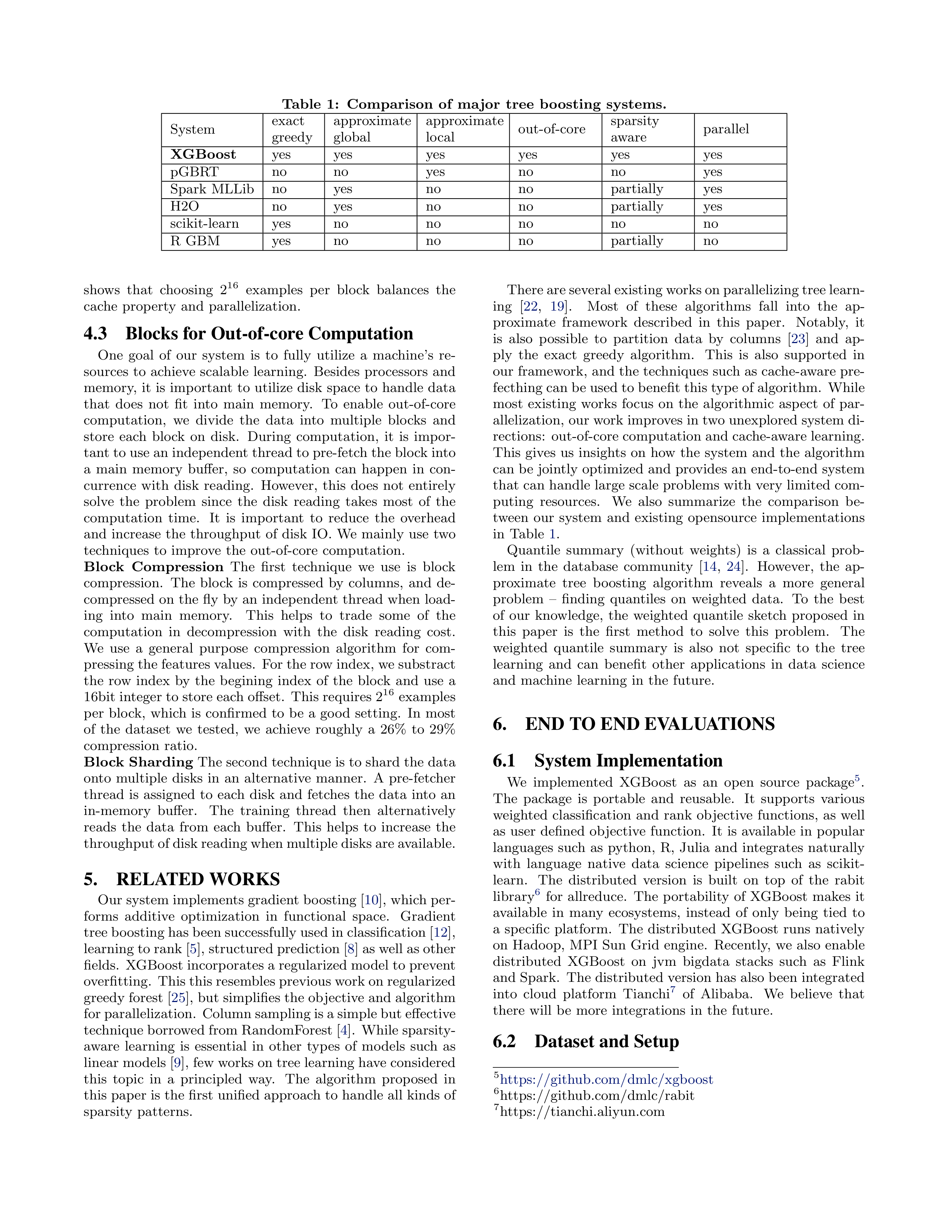
],
It
is
implemented
in
a
commercial
software
TreeNet
4
for
gradient
boosting,
but
is
not
implemented
in
existing
opensource packages.
According to user feedback,
using col-
umn
sub-sampling
prevents
over-fitting
even
more
so
than
the
traditional
row
sub-sampling
(which
is
also
supported).
The
usage
of
column
sub-samples
also
speeds
up
computa-
tions
of
the
parallel
algorithm
described
later.
3.
SPLIT FINDING ALGORITHMS
3.1
Basic Exact Greedy Algorithm
One
of
the
key
problems
in
tree
learning
is
to
find
the
best
split
as
indicated
by
Eq
(
7
).
In
order
to
do
so,
a
split
finding
algorithm
enumerates
over
all
the
possible
splits
on
all
the
features.
We
call
this
the
exact
greedy
algorithm
.
Most existing single machine tree boosting implementations,
such
as
scikit-learn
[
20
],
R’s
gbm
[
21
]
as
well
as
the
single
machine
version
of
XGBoost
support
the
exact
greedy
algo-
rithm.
The
exact
greedy
algorithm
is
shown
in
Alg.
1
.
It
is
computationally
demanding
to
enumerate
all
the
possible
splits
for
continuous
features.
In
order
to
do
so
efficiently,
the
algorithm
must
first
sort
the
data
according
to
feature
values
and
visit
the
data
in
sorted
order
to
accumulate
the
gradient
statistics
for
the
structure
score
in
Eq
(
7
).
3.2
Approximate Algorithm
The
exact
greedy
algorithm
is
very
powerful
since
it
enu-
merates
over
all
possible
splitting
points
greedily.
However,
it is impossible to efficiently do so when the data does not fit
entirely
into
memory.
Same
problem
also
arises
in
the
dis-
4
https://www.salford-systems.com/products/treenet
0
10
20
30
40
50
60
70
80
90
Number of Iterations
0
.
75
0
.
76
0
.
77
0
.
78
0
.
79
0
.
80
0
.
81
0
.
82
0
.
83
Test AUC
exact greedy
global eps=0.3
local eps=0.3
global eps=0.05
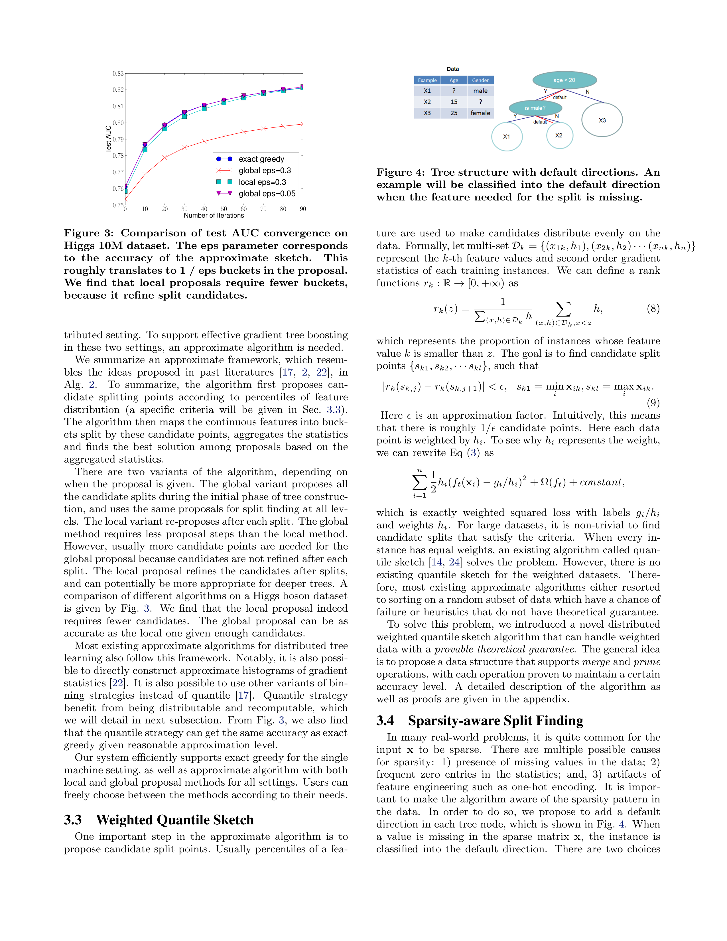
Figure
3:
Comparison
of
test
AUC
convergence
on
Higgs
10M
dataset.
The
eps
parameter
corresponds
to
the
accuracy
of
the
approximate
sketch.
This
roughly translates to 1 / eps buckets in the proposal.
We
find
that
local
proposals
require
fewer
buckets,
because
it
refine
split
candidates.
tributed setting.
To support effective gradient tree boosting
in
these
two
settings,
an
approximate
algorithm
is
needed.
We
summarize
an
approximate
framework,
which
resem-
bles
the
ideas
proposed
in
past
literatures
[
17
,
2
,
22
],
in
Alg.
2
.
To
summarize,
the
algorithm
first
proposes
can-
didate
splitting
points
according
to
percentiles
of
feature
distribution
(a
specific
criteria
will
be
given
in
Sec.
3.3
).
The algorithm then maps the continuous features into buck-
ets
split
by
these
candidate
points,
aggregates
the
statistics
and
finds
the
best
solution
among
proposals
based
on
the
aggregated
statistics.
There
are
two
variants
of
the
algorithm,
depending
on
when
the
proposal
is
given.
The
global
variant
proposes
all
the candidate splits during the initial phase of tree construc-
tion,
and
uses
the
same
proposals
for
split
finding
at
all
lev-
els.
The local variant re-proposes after each split.
The global
method
requires
less
proposal
steps
than
the
local
method.
However,
usually
more
candidate
points
are
needed
for
the
global proposal because candidates are not refined after each
split.
The
local
proposal
refines
the
candidates
after
splits,
and can potentially be more appropriate for deeper trees.
A
comparison of different algorithms on a Higgs boson dataset
is
given
by
Fig.
3
.
We
find
that
the
local
proposal
indeed
requires
fewer
candidates.
The
global
proposal
can
be
as
accurate
as
the
local
one
given
enough
candidates.
Most existing approximate algorithms for distributed tree
learning also follow this framework.
Notably, it is also possi-
ble to directly construct approximate histograms of gradient
statistics [
22
].
It is also possible to use other variants of bin-
ning
strategies
instead
of
quantile
[
17
].
Quantile
strategy
benefit
from
being
distributable
and
recomputable,
which
we
will
detail
in
next
subsection.
From
Fig.
3
,
we
also
find
that the quantile strategy can get the same accuracy as exact
greedy
given
reasonable
approximation
level.
Our system efficiently supports exact greedy for the single
machine setting, as well as approximate algorithm with both
local and global proposal methods for all settings.
Users can
freely choose between the
methods
according to
their needs.
3.3
Weighted Quantile Sketch
One
important
step
in
the
approximate
algorithm
is
to
propose
candidate
split
points.
Usually
percentiles
of
a
fea-
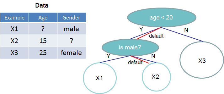
Figure
4:
Tree
structure
with
default
directions.
An
example
will
be
classified
into
the
default
direction
when
the
feature
needed
for
the
split
is
missing.
ture
are
used
to
make
candidates
distribute
evenly
on
the
data.
Formally, let multi-set
D
k
=
{
(
x
1
k
, h
1
)
,
(
x
2
k
, h
2
)
· · ·
(
x
nk
, h
n
)
}
represent
the
k
-th
feature
values
and
second
order
gradient
statistics
of
each
training
instances.
We
can
define
a
rank
functions
r
k
:
R
→
[0
,
+
∞
)
as
r
k
(
z
) =
1
P
(
x,h
)
∈D
k
h
X
(
x,h
)
∈D
k
,x<z
h,
(8)
which
represents
the
proportion
of
instances
whose
feature
value
k
is
smaller
than
z
.
The
goal
is
to
find
candidate
split
points
{
s
k
1
, s
k
2
,
· · ·
s
kl
}
,
such
that
|
r
k
(
s
k,j
)
−
r
k
(
s
k,j
+1
)
|
< ϵ,
s
k
1
= min
i
x
ik
, s
kl
= max
i
x
ik
.
(9)
Here
ϵ
is
an
approximation
factor.
Intuitively,
this
means
that
there
is
roughly
1
/ϵ
candidate
points.
Here
each
data
point is weighted by
h
i
.
To see why
h
i
represents the weight,
we
can
rewrite
Eq
(
3
)
as
n
X
i
=1
1
2
h
i
(
f
t
(
x
i
)
−
g
i
/h
i
)
2
+ Ω(
f
t
) +
constant,
which
is
exactly
weighted
squared
loss
with
labels
g
i
/h
i
and
weights
h
i
.
For
large
datasets,
it
is
non-trivial
to
find
candidate
splits
that
satisfy
the
criteria.
When
every
in-
stance
has
equal
weights,
an
existing
algorithm
called
quan-
tile
sketch
[
14
,
24
]
solves
the
problem.
However,
there
is
no
existing
quantile
sketch
for
the
weighted
datasets.
There-
fore,
most
existing
approximate
algorithms
either
resorted
to sorting on a random subset of data which have a chance of
failure
or
heuristics
that
do
not
have
theoretical
guarantee.
To
solve
this
problem,
we
introduced
a
novel
distributed
weighted quantile sketch algorithm that can handle weighted
data
with
a
provable
theoretical
guarantee
.
The
general
idea
is to propose a data structure that supports
merge
and
prune
operations, with each operation proven to maintain a certain
accuracy
level.
A
detailed
description
of
the
algorithm
as
well
as
proofs
are
given
in
the
appendix.
3.4
Sparsity-aware Split Finding
In
many
real-world
problems,
it
is
quite
common
for
the
input
x
to
be
sparse.
There
are
multiple
possible
causes
for
sparsity:
1)
presence
of
missing
values
in
the
data;
2)
frequent
zero
entries
in
the
statistics;
and,
3)
artifacts
of
feature
engineering
such
as
one-hot
encoding.
It
is
impor-
tant
to
make
the
algorithm
aware
of
the
sparsity
pattern
in
the
data.
In
order
to
do
so,
we
propose
to
add
a
default
direction
in
each
tree
node,
which
is
shown
in
Fig.
4
.
When
a
value
is
missing
in
the
sparse
matrix
x
,
the
instance
is
classified
into
the
default
direction.
There
are
two
choices
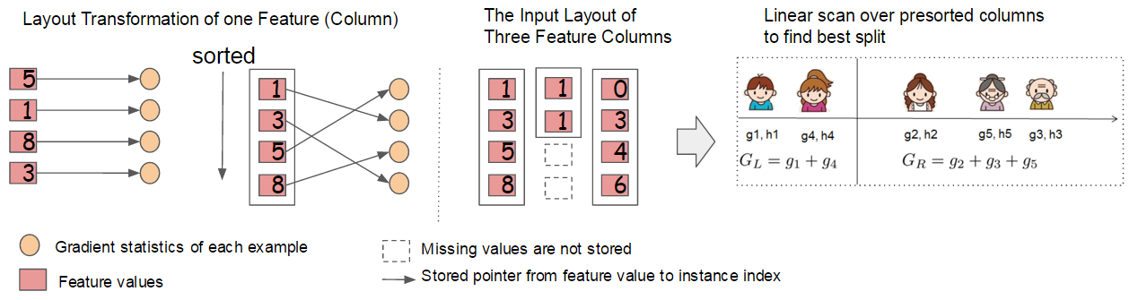
Figure
6:
Block
structure
for
parallel
learning.
Each
column
in
a
block
is
sorted
by
the
corresponding
feature
value.
A
linear
scan
over
one
column
in
the
block
is
sufficient
to
enumerate
all
the
split
points.
Algorithm
3:
Sparsity-aware
Split
Finding
Input
:
I
,
instance
set
of
current
node
Input
:
I
k
=
{
i
∈
I
|
x
ik
̸
= missing
}
Input
:
d
,
feature
dimension
Also
applies
to
the
approximate
setting,
only
collect
statistics
of
non-missing
entries
into
buckets
gain
←
0
G
←
P
i
∈
I
, g
i
,
H
←
P
i
∈
I
h
i
for
k
= 1
to
m
do
//
enumerate
missing
value
goto
right
G
L
←
0
,
H
L
←
0
for
j
in
sorted(
I
k
,
ascent
order
by
x
jk
)
do
G
L
←
G
L
+
g
j
,
H
L
←
H
L
+
h
j
G
R
←
G
−
G
L
,
H
R
←
H
−
H
L
score
←
max(
score,
G
2
L
H
L
+
λ
+
G
2
R
H
R
+
λ
−
G
2
H
+
λ
)
end
//
enumerate
missing
value
goto
left
G
R
←
0
,
H
R
←
0
for
j
in
sorted(
I
k
,
descent
order
by
x
jk
)
do
G
R
←
G
R
+
g
j
,
H
R
←
H
R
+
h
j
G
L
←
G
−
G
R
,
H
L
←
H
−
H
R
score
←
max(
score,
G
2
L
H
L
+
λ
+
G
2
R
H
R
+
λ
−
G
2
H
+
λ
)
end
end
Output
:
Split
and
default
directions
with
max
gain
of
default
direction
in
each
branch.
The
optimal
default
di-
rections are learnt from the data.
The algorithm is shown in
Alg.
3
.
The key improvement is to only visit the non-missing
entries
I
k
.
The
presented
algorithm
treats
the
non-presence
as
a
missing
value
and
learns
the
best
direction
to
handle
missing
values.
The
same
algorithm
can
also
be
applied
when
the
non-presence
corresponds
to
a
user
specified
value
by
limiting
the
enumeration
only
to
consistent
solutions.
To
the
best
of
our
knowledge,
most
existing
tree
learn-
ing
algorithms
are
either
only
optimized
for
dense
data,
or
need specific procedures
to
handle
limited cases
such as cat-
egorical
encoding.
XGBoost
handles
all
sparsity
patterns
in
a
unified
way.
More
importantly,
our
method
exploits
the
sparsity
to
make
computation
complexity
linear
to
number
of
non-missing
entries
in
the
input.
Fig.
5
shows
the
com-
parison
of
sparsity
aware
and
a
naive
implementation
on
an
Allstate-10K dataset (description of dataset given in Sec.
6
).
We
find
that
the
sparsity
aware
algorithm
runs
50
times
faster
than
the
naive
version.
This
confirms
the
importance
of
the
sparsity
aware
algorithm.
1
2
4
8
16
Number of Threads
0.03125
0.0625
0.125
0.25
0.5
1
2
4
8
16
32
Time per Tree(sec)
Sparsity aware algorithm
Basic algorithm
Figure
5:
Impact
of
the
sparsity
aware
algorithm
on
Allstate-10K.
The
dataset
is
sparse
mainly
due
to
one-hot
encoding.
The
sparsity
aware
algorithm
is
more
than
50
times
faster
than
the
naive
version
that
does
not
take
sparsity
into
consideration.
4.
SYSTEM DESIGN
4.1
Column Block for Parallel Learning
The
most
time
consuming
part
of
tree
learning
is
to
get
the
data
into
sorted
order.
In
order
to
reduce
the
cost
of
sorting,
we
propose
to
store
the
data
in
in-memory
units,
which
we
called
block
.
Data
in
each
block
is
stored
in
the
compressed
column
(CSC)
format,
with
each
column
sorted
by
the
corresponding
feature
value.
This
input
data
layout
only
needs
to
be
computed
once
before
training,
and
can
be
reused
in
later
iterations.
In
the
exact
greedy
algorithm,
we
store
the
entire
dataset
in
a
single
block
and
run
the
split
search
algorithm
by
lin-
early
scanning
over
the
pre-sorted
entries.
We
do
the
split
finding
of
all
leaves
collectively,
so
one
scan
over
the
block
will
collect
the
statistics
of
the
split
candidates
in
all
leaf
branches.
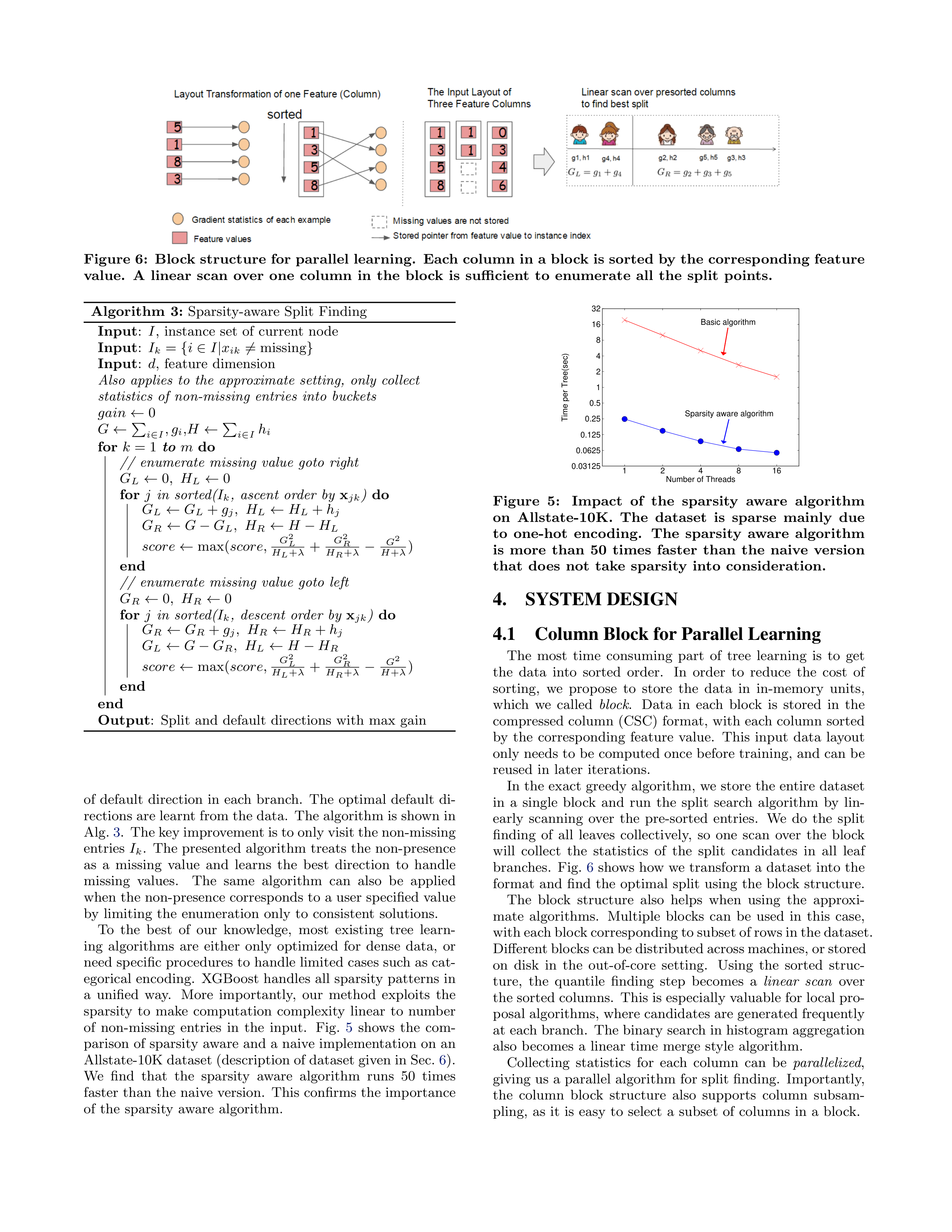
Fig.
6
shows
how
we
transform
a
dataset
into
the
format
and
find
the
optimal
split
using
the
block
structure.
The
block
structure
also
helps
when
using
the
approxi-
mate
algorithms.
Multiple
blocks
can
be
used
in
this
case,
with each block corresponding to subset of rows in the dataset.
Different blocks can be distributed across machines, or stored
on
disk
in
the
out-of-core
setting.
Using
the
sorted
struc-
ture,
the
quantile
finding
step
becomes
a
linear
scan
over
the sorted columns.
This is especially valuable for local pro-
posal algorithms, where candidates are generated frequently
at each branch.
The binary search in histogram aggregation
also
becomes
a
linear
time
merge
style
algorithm.
Collecting
statistics
for
each
column
can
be
parallelized
,
giving
us
a
parallel
algorithm
for
split
finding.
Importantly,
the
column
block
structure
also
supports
column
subsam-
pling,
as
it
is
easy
to
select
a
subset
of
columns
in
a
block.
1
2
4
8
16
Number of Threads
8
16
32
64
128
Time per Tree(sec)
Basic algorithm
Cache-aware algorithm
(a)
Allstate
10M
1
2
4
8
16
Number of Threads
8
16
32
64
128
256
Time per Tree(sec)
Basic algorithm
Cache-aware algorithm
(b)
Higgs
10M
1
2
4
8
16
Number of Threads
0.25
0.5
1
2
4
8
Time per Tree(sec)
Basic algorithm
Cache-aware algorithm
(c)
Allstate
1M
1
2
4
8
16
Number of Threads
0.25
0.5
1
2
4
8
Time per Tree(sec)
Basic algorithm
Cache-aware algorithm
(d)
Higgs
1M
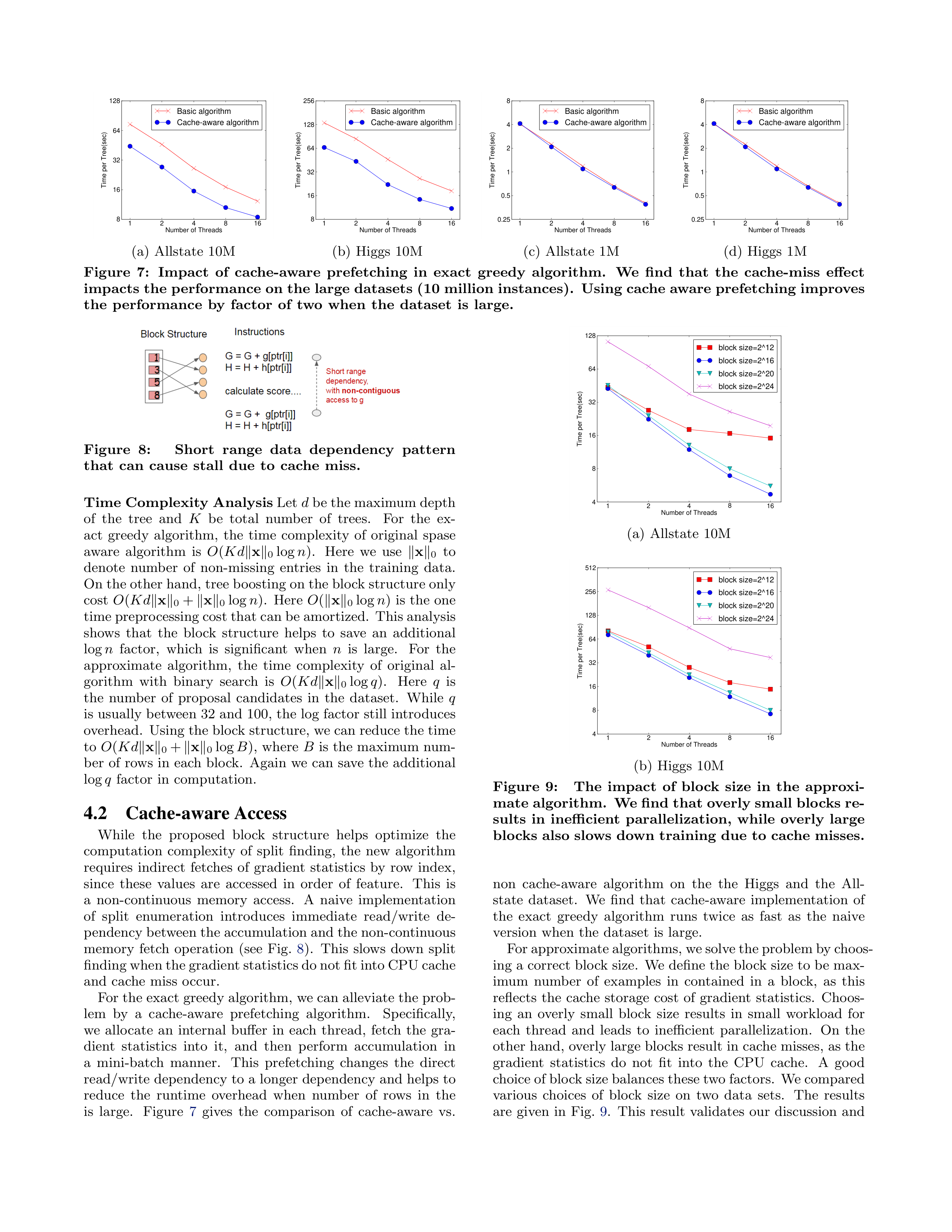
Figure
7:
Impact
of
cache-aware
prefetching
in
exact
greedy
algorithm.
We
find
that
the
cache-miss
effect
impacts
the
performance
on
the
large
datasets
(10
million
instances).
Using
cache
aware
prefetching
improves
the
performance
by
factor
of
two
when
the
dataset
is
large.
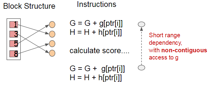
Figure
8:
Short
range
data
dependency
pattern
that
can
cause
stall
due
to
cache
miss.
Time Complexity
Analysis
Let
d
be the maximum depth
of
the
tree
and
K
be
total
number
of
trees.
For
the
ex-
act
greedy
algorithm,
the
time
complexity
of
original
spase
aware
algorithm
is
O
(
Kd
∥
x
∥
0
log
n
).
Here
we
use
∥
x
∥
0
to
denote
number
of
non-missing
entries
in
the
training
data.
On the other hand, tree boosting on the block structure only
cost
O
(
Kd
∥
x
∥
0
+
∥
x
∥
0
log
n
).
Here
O
(
∥
x
∥
0
log
n
)
is
the
one
time preprocessing cost that can be amortized.
This analysis
shows
that
the
block
structure
helps
to
save
an
additional
log
n
factor,
which
is
significant
when
n
is
large.
For
the
approximate
algorithm,
the
time
complexity
of
original
al-
gorithm
with
binary
search
is
O
(
Kd
∥
x
∥
0
log
q
).
Here
q
is
the
number
of
proposal
candidates
in
the
dataset.
While
q
is
usually
between
32
and
100,
the
log
factor
still
introduces
overhead.
Using the block structure, we can reduce the time
to
O
(
Kd
∥
x
∥
0
+
∥
x
∥
0
log
B
),
where
B
is
the
maximum
num-
ber
of
rows
in
each
block.
Again
we
can
save
the
additional
log
q
factor
in
computation.
4.2
Cache-aware Access
While
the
proposed
block
structure
helps
optimize
the
computation
complexity
of
split
finding,
the
new
algorithm
requires
indirect
fetches
of
gradient
statistics
by
row
index,
since
these
values
are
accessed
in
order
of
feature.
This
is
a
non-continuous
memory
access.
A
naive
implementation
of
split
enumeration
introduces
immediate
read/write
de-
pendency between the accumulation and the non-continuous
memory
fetch
operation
(see
Fig.
8
).
This
slows
down
split
finding when the gradient statistics do not fit into CPU cache
and
cache
miss
occur.
For the exact greedy algorithm, we can alleviate the prob-
lem
by
a
cache-aware
prefetching
algorithm.
Specifically,
we
allocate
an
internal
buffer
in
each
thread,
fetch
the
gra-
dient
statistics
into
it,
and
then
perform
accumulation
in
a
mini-batch
manner.
This
prefetching
changes
the
direct
read/write
dependency
to
a
longer
dependency
and
helps
to
reduce
the
runtime
overhead
when
number
of
rows
in
the
is
large.
Figure
7
gives
the
comparison
of
cache-aware
vs.
1
2
4
8
16
Number of Threads
4
8
16
32
64
128
Time per Tree(sec)
block size=2^12
block size=2^16
block size=2^20
block size=2^24
(a)
Allstate
10M
1
2
4
8
16
Number of Threads
4
8
16
32
64
128
256
512
Time per Tree(sec)
block size=2^12
block size=2^16
block size=2^20
block size=2^24
(b)
Higgs
10M
Figure
9:
The
impact
of
block
size
in
the
approxi-
mate algorithm.
We find that overly small blocks re-
sults
in
inefficient
parallelization,
while
overly
large
blocks
also
slows
down
training
due
to
cache
misses.
non
cache-aware
algorithm
on
the
the
Higgs
and
the
All-
state
dataset.
We
find
that
cache-aware
implementation
of
the
exact
greedy
algorithm
runs
twice
as
fast
as
the
naive
version
when
the
dataset
is
large.
For approximate algorithms, we solve the problem by choos-
ing
a
correct
block
size.
We
define
the
block
size
to
be
max-
imum
number
of
examples
in
contained
in
a
block,
as
this
reflects
the
cache
storage
cost
of
gradient
statistics.
Choos-
ing
an
overly
small
block
size
results
in
small
workload
for
each
thread
and
leads
to
inefficient
parallelization.
On
the
other hand,
overly large blocks result in cache misses,
as the
gradient
statistics
do
not
fit
into
the
CPU
cache.
A
good
choice of block size balances these two factors.
We compared
various
choices
of
block
size
on
two
data
sets.
The
results
are
given
in
Fig.
9
.
This
result
validates
our
discussion
and
Table
1:
Comparison
of
major
tree
boosting
systems.
System
exact
greedy
approximate
global
approximate
local
out-of-core
sparsity
aware
parallel
XGBoost
yes
yes
yes
yes
yes
yes
pGBRT
no
no
yes
no
no
yes
Spark
MLLib
no
yes
no
no
partially
yes
H2O
no
yes
no
no
partially
yes
scikit-learn
yes
no
no
no
no
no
R
GBM
yes
no
no
no
partially
no
shows
that
choosing
2
16
examples
per
block
balances
the
cache
property
and
parallelization.
4.3
Blocks for Out-of-core Computation
One
goal
of
our
system
is
to
fully
utilize
a
machine’s
re-
sources
to
achieve
scalable
learning.
Besides
processors
and
memory,
it
is
important
to
utilize
disk
space
to
handle
data
that
does
not
fit
into
main
memory.
To
enable
out-of-core
computation,
we
divide
the
data
into
multiple
blocks
and
store
each
block
on
disk.
During
computation,
it
is
impor-
tant to use an independent thread to pre-fetch the block into
a
main
memory
buffer,
so
computation
can
happen
in
con-
currence
with
disk
reading.
However,
this
does
not
entirely
solve
the
problem
since
the
disk
reading
takes
most
of
the
computation
time.
It
is
important
to
reduce
the
overhead
and
increase
the
throughput
of
disk
IO.
We
mainly
use
two
techniques
to
improve
the
out-of-core
computation.
Block
Compression
The
first
technique
we
use
is
block
compression.
The
block
is
compressed
by
columns,
and
de-
compressed
on
the
fly
by
an
independent
thread
when
load-
ing
into
main
memory.
This
helps
to
trade
some
of
the
computation
in
decompression
with
the
disk
reading
cost.
We
use
a
general
purpose
compression
algorithm
for
com-
pressing the features values.
For the row index, we substract
the
row
index
by
the
begining
index
of
the
block
and
use
a
16bit integer to store each offset.
This requires 2
16
examples
per
block,
which
is
confirmed
to
be
a
good
setting.
In
most
of
the
dataset
we
tested,
we
achieve
roughly
a
26%
to
29%
compression
ratio.
Block
Sharding
The second technique is to shard the data
onto
multiple
disks
in
an
alternative
manner.
A
pre-fetcher
thread
is
assigned
to
each
disk
and
fetches
the
data
into
an
in-memory
buffer.
The
training
thread
then
alternatively
reads
the
data
from
each
buffer.
This
helps
to
increase
the
throughput of disk reading when multiple disks are available.
5.
RELATED WORKS
Our system implements gradient boosting [
10
], which per-
forms
additive
optimization
in
functional
space.
Gradient
tree boosting has been successfully used in classification [
12
],
learning to rank [
5
], structured prediction [
8
] as well as other
fields.
XGBoost incorporates a regularized model to prevent
overfitting.
This this resembles previous work on regularized
greedy forest [
25
], but simplifies the objective and algorithm
for parallelization.
Column sampling is a simple but effective
technique borrowed from RandomForest [
4
].
While sparsity-
aware
learning
is
essential
in
other
types
of
models
such
as
linear models [
9
], few works on tree learning have considered
this
topic
in
a
principled
way.
The
algorithm
proposed
in
this
paper
is
the
first
unified
approach
to
handle
all
kinds
of
sparsity
patterns.
There are several existing works on parallelizing tree learn-
ing
[
22
,
19
].
Most
of
these
algorithms
fall
into
the
ap-
proximate
framework
described
in
this
paper.
Notably,
it
is
also
possible
to
partition
data
by
columns
[
23
]
and
ap-
ply
the
exact
greedy
algorithm.
This
is
also
supported
in
our
framework,
and
the
techniques
such
as
cache-aware
pre-
fecthing can be used to benefit this type of algorithm.
While
most
existing
works
focus
on
the
algorithmic
aspect
of
par-
allelization, our work improves in two unexplored system di-
rections:
out-of-core computation and cache-aware learning.
This
gives
us
insights
on
how
the
system
and
the
algorithm
can
be
jointly
optimized
and
provides
an
end-to-end
system
that
can
handle
large
scale
problems
with
very
limited
com-
puting
resources.
We
also
summarize
the
comparison
be-
tween
our
system
and
existing
opensource
implementations
in
Table
1
.
Quantile
summary
(without
weights)
is
a
classical
prob-
lem
in
the
database
community
[
14
,
24
].
However,
the
ap-
proximate
tree
boosting
algorithm
reveals
a
more
general
problem
–
finding
quantiles
on
weighted
data.
To
the
best
of
our
knowledge,
the
weighted
quantile
sketch
proposed
in
this
paper
is
the
first
method
to
solve
this
problem.
The
weighted
quantile
summary
is
also
not
specific
to
the
tree
learning
and
can
benefit
other
applications
in
data
science
and
machine
learning
in
the
future.
6.
END TO END EVALUATIONS
6.1
System Implementation
We
implemented
XGBoost
as
an
open
source
package
5
.
The
package
is
portable
and
reusable.
It
supports
various
weighted
classification
and
rank
objective
functions,
as
well
as
user
defined
objective
function.
It
is
available
in
popular
languages
such
as
python,
R,
Julia
and
integrates
naturally
with
language
native
data
science
pipelines
such
as
scikit-
learn.
The
distributed
version
is
built
on
top
of
the
rabit
library
6
for
allreduce.
The
portability
of
XGBoost
makes
it
available
in
many
ecosystems,
instead
of
only
being
tied
to
a
specific
platform.
The
distributed
XGBoost
runs
natively
on
Hadoop,
MPI
Sun
Grid
engine.
Recently,
we
also
enable
distributed
XGBoost
on
jvm
bigdata
stacks
such
as
Flink
and Spark.
The distributed version has also been integrated
into
cloud
platform
Tianchi
7
of
Alibaba.
We
believe
that
there
will
be
more
integrations
in
the
future.
6.2
Dataset and Setup
5
https://github.com/dmlc/xgboost
6
https://github.com/dmlc/rabit
7
https://tianchi.aliyun.com
Table
2:
Dataset
used
in
the
Experiments.
Dataset
n
m
Task
Allstate
10
M
4227
Insurance
claim
classification
Higgs
Boson
10
M
28
Event
classification
Yahoo
LTRC
473K
700
Learning
to
Rank
Criteo
1.7
B
67
Click
through
rate
prediction
We
used
four
datasets
in
our
experiments.
A
summary
of
these
datasets
is
given
in
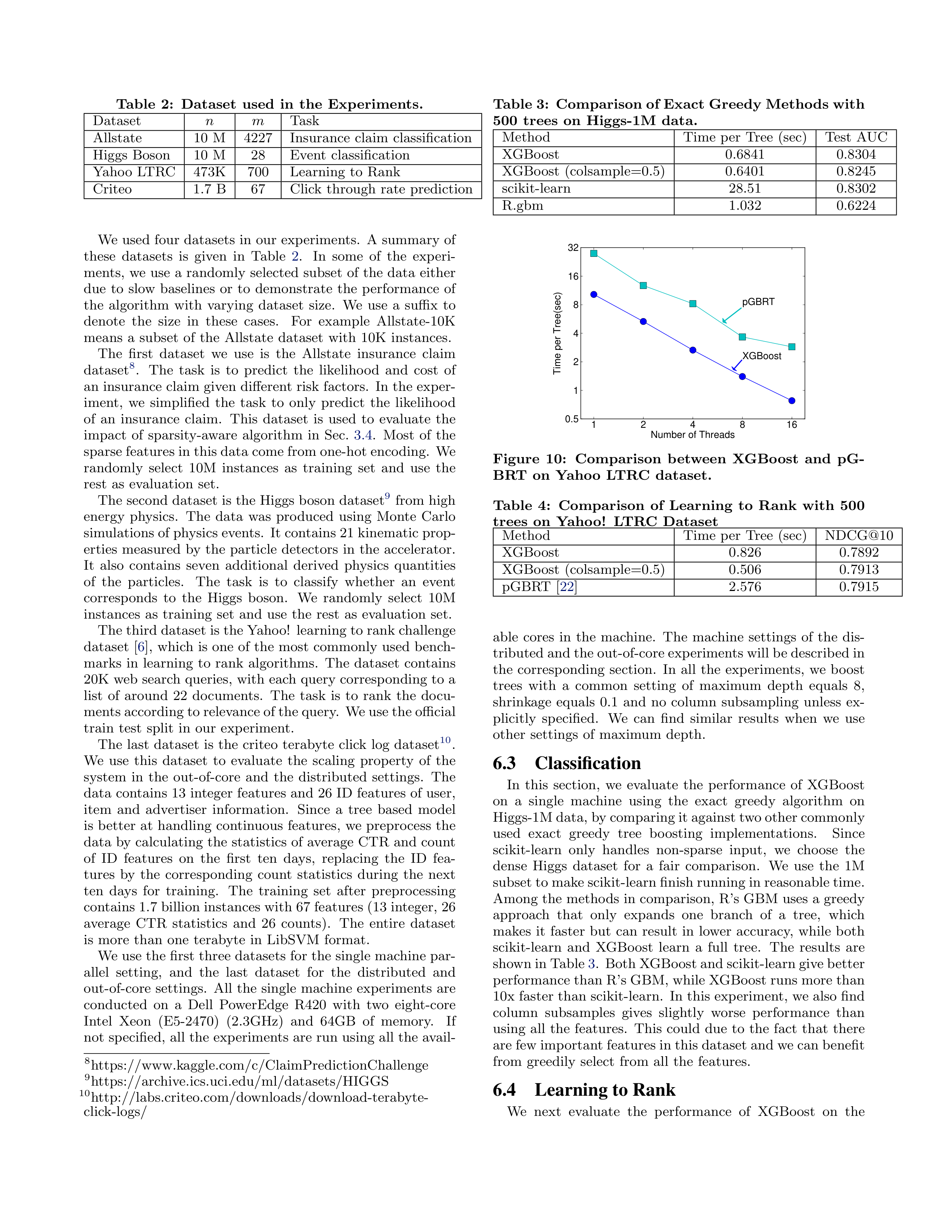
Table
2
.
In
some
of
the
experi-
ments,
we
use
a
randomly
selected
subset
of
the
data
either
due
to
slow
baselines
or
to
demonstrate
the
performance
of
the
algorithm
with
varying
dataset
size.
We
use
a
suffix
to
denote
the
size
in
these
cases.
For
example
Allstate-10K
means
a
subset
of
the
Allstate
dataset
with
10K
instances.
The
first
dataset
we
use
is
the
Allstate
insurance
claim
dataset
8
.
The
task
is
to
predict
the
likelihood
and
cost
of
an insurance claim given different risk factors.
In the exper-
iment,
we
simplified
the
task
to
only
predict
the
likelihood
of
an
insurance
claim.
This
dataset
is
used
to
evaluate
the
impact
of
sparsity-aware
algorithm
in
Sec.
3.4
.
Most
of
the
sparse features in this data come from one-hot encoding.
We
randomly
select
10M
instances
as
training
set
and
use
the
rest
as
evaluation
set.
The
second
dataset
is
the
Higgs
boson
dataset
9
from
high
energy
physics.
The
data
was
produced
using
Monte
Carlo
simulations of physics events.
It contains 21 kinematic prop-
erties
measured
by
the
particle
detectors
in
the
accelerator.
It
also
contains
seven
additional
derived
physics
quantities
of
the
particles.
The
task
is
to
classify
whether
an
event
corresponds
to
the
Higgs
boson.
We
randomly
select
10M
instances
as
training
set
and
use
the
rest
as
evaluation
set.
The third dataset is the Yahoo!
learning to rank challenge
dataset
[
6
],
which
is
one
of
the
most
commonly
used
bench-
marks
in
learning
to
rank
algorithms.
The
dataset
contains
20K
web
search
queries,
with
each
query
corresponding
to
a
list
of
around
22
documents.
The
task
is
to
rank
the
docu-
ments according to relevance of the query.
We use the official
train
test
split
in
our
experiment.
The
last
dataset
is
the
criteo
terabyte
click
log
dataset
10
.
We
use
this
dataset
to
evaluate
the
scaling
property
of
the
system
in
the
out-of-core
and
the
distributed
settings.
The
data
contains
13
integer
features
and
26
ID
features
of
user,
item
and
advertiser
information.
Since
a
tree
based
model
is
better
at
handling
continuous
features,
we
preprocess
the
data
by
calculating
the
statistics
of
average
CTR
and
count
of
ID
features
on
the
first
ten
days,
replacing
the
ID
fea-
tures
by
the
corresponding
count
statistics
during
the
next
ten
days
for
training.
The
training
set
after
preprocessing
contains 1.7 billion instances with 67 features (13 integer, 26
average
CTR
statistics
and
26
counts).
The
entire
dataset
is
more
than
one
terabyte
in
LibSVM
format.
We use the first three datasets for the single machine par-
allel
setting,
and
the
last
dataset
for
the
distributed
and
out-of-core
settings.
All
the
single
machine
experiments
are
conducted
on
a
Dell
PowerEdge
R420
with
two
eight-core
Intel
Xeon
(E5-2470)
(2.3GHz)
and
64GB
of
memory.
If
not
specified,
all
the
experiments
are
run
using
all
the
avail-
8
https://www.kaggle.com/c/ClaimPredictionChallenge
9
https://archive.ics.uci.edu/ml/datasets/HIGGS
10
http://labs.criteo.com/downloads/download-terabyte-
click-logs/
Table 3:
Comparison of Exact Greedy Methods with
500
trees
on
Higgs-1M
data.
Method
Time
per
Tree
(sec)
Test
AUC
XGBoost
0.6841
0.8304
XGBoost
(colsample=0.5)
0.6401
0.8245
scikit-learn
28.51
0.8302
R.gbm
1.032
0.6224
1
2
4
8
16
Number of Threads
0.5
1
2
4
8
16
32
Time per Tree(sec)
XGBoost
pGBRT
Figure
10:
Comparison
between
XGBoost
and
pG-
BRT
on
Yahoo
LTRC
dataset.
Table
4:
Comparison
of
Learning
to
Rank
with
500
trees
on
Yahoo!
LTRC
Dataset
Method
Time
per
Tree
(sec)
NDCG@10
XGBoost
0.826
0.7892
XGBoost
(colsample=0.5)
0.506
0.7913
pGBRT
[
22
]
2.576
0.7915
able
cores
in
the
machine.
The
machine
settings
of
the
dis-
tributed and the out-of-core experiments will be described in
the
corresponding
section.
In
all
the
experiments,
we
boost
trees
with
a
common
setting
of
maximum
depth
equals
8,
shrinkage
equals
0.1
and
no
column
subsampling
unless
ex-
plicitly
specified.
We
can
find
similar
results
when
we
use
other
settings
of
maximum
depth.
6.3
Classification
In
this
section,
we
evaluate
the
performance
of
XGBoost
on
a
single
machine
using
the
exact
greedy
algorithm
on
Higgs-1M data, by comparing it against two other commonly
used
exact
greedy
tree
boosting
implementations.
Since
scikit-learn
only
handles
non-sparse
input,
we
choose
the
dense
Higgs
dataset
for
a
fair
comparison.
We
use
the
1M
subset to make scikit-learn finish running in reasonable time.
Among
the
methods
in
comparison,
R’s
GBM
uses
a
greedy
approach
that
only
expands
one
branch
of
a
tree,
which
makes
it
faster
but
can
result
in
lower
accuracy,
while
both
scikit-learn
and
XGBoost
learn
a
full
tree.
The
results
are
shown in Table
3
.
Both XGBoost and scikit-learn give better
performance than R’s GBM, while XGBoost runs more than
10x faster
than scikit-learn.
In this experiment,
we
also
find
column
subsamples
gives
slightly
worse
performance
than
using
all
the
features.
This
could
due
to
the
fact
that
there
are few important features in this dataset and we can benefit
from
greedily
select
from
all
the
features.
6.4
Learning to Rank
We
next
evaluate
the
performance
of
XGBoost
on
the
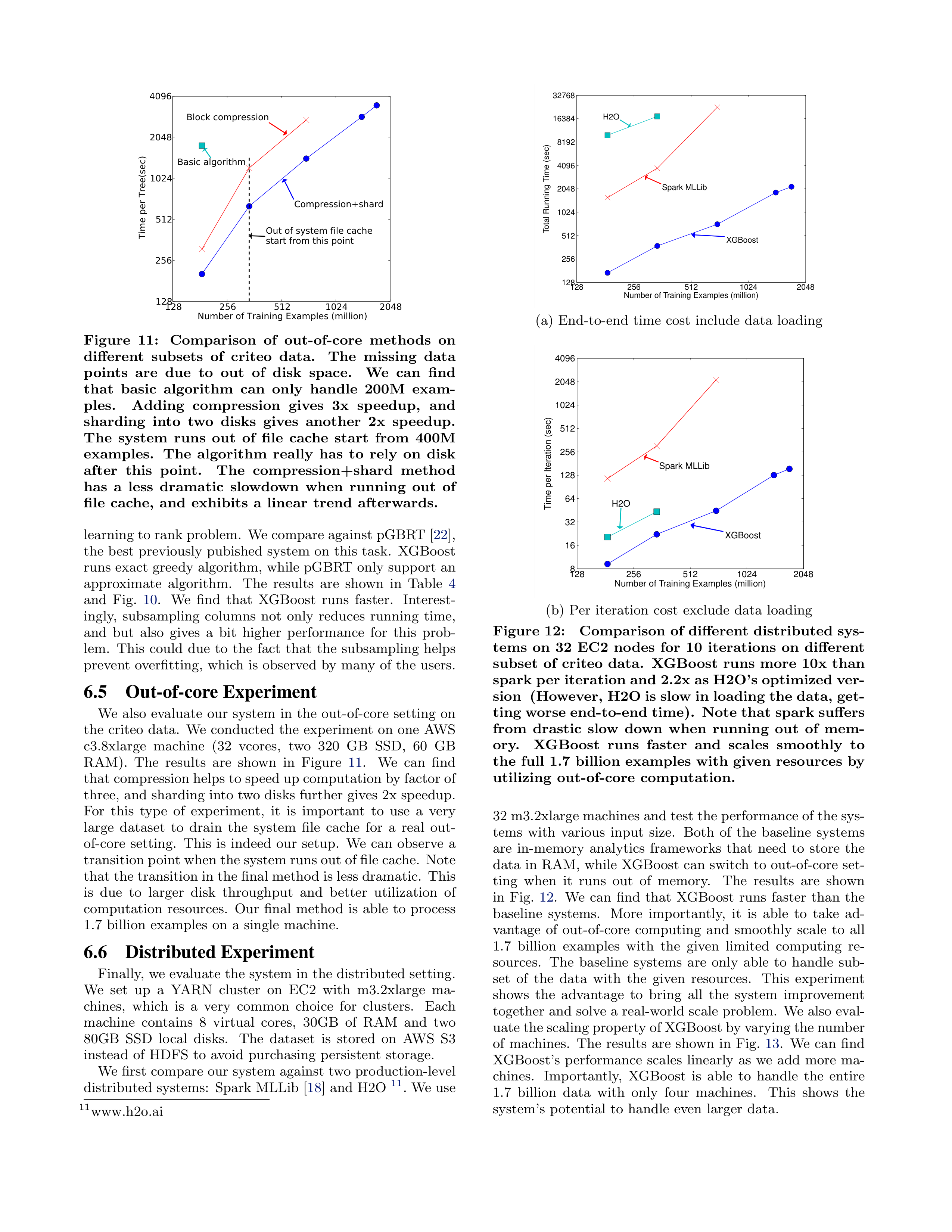
128
256
512
1024
2048
Number of Training Examples (million)
128
256
512
1024
2048
4096
Time per Tree(sec)
Basic algorithm
Block compression
Compression+shard
Out of system file cache
start from this point
Figure
11:
Comparison
of
out-of-core
methods
on
different
subsets
of
criteo
data.
The
missing
data
points
are
due
to
out
of
disk
space.
We
can
find
that
basic
algorithm
can
only
handle
200M
exam-
ples.
Adding
compression
gives
3x
speedup,
and
sharding
into
two
disks
gives
another
2x
speedup.
The
system
runs
out
of
file
cache
start
from
400M
examples.
The
algorithm
really
has
to
rely
on
disk
after
this
point.
The
compression+shard
method
has
a
less
dramatic
slowdown
when
running
out
of
file
cache,
and
exhibits
a
linear
trend
afterwards.
learning to rank problem.
We compare against pGBRT [
22
],
the
best
previously
pubished
system
on
this
task.
XGBoost
runs
exact
greedy
algorithm,
while
pGBRT
only
support
an
approximate
algorithm.
The
results
are
shown
in
Table
4
and
Fig.
10
.
We
find
that
XGBoost
runs
faster.
Interest-
ingly,
subsampling
columns
not
only
reduces
running
time,
and
but
also
gives
a
bit
higher
performance
for
this
prob-
lem.
This
could
due
to
the
fact
that
the
subsampling
helps
prevent
overfitting,
which
is
observed
by
many
of
the
users.
6.5
Out-of-core Experiment
We
also
evaluate
our
system
in
the
out-of-core
setting
on
the
criteo
data.
We
conducted
the
experiment
on
one
AWS
c3.8xlarge
machine
(32
vcores,
two
320
GB
SSD,
60
GB
RAM).
The
results
are
shown
in
Figure
11
.
We
can
find
that compression helps to speed up computation by factor of
three,
and
sharding
into
two
disks
further
gives
2x
speedup.
For
this
type
of
experiment,
it
is
important
to
use
a
very
large
dataset
to
drain
the
system
file
cache
for
a
real
out-
of-core
setting.
This
is
indeed
our
setup.
We
can
observe
a
transition point when the system runs out of file cache.
Note
that the transition in the final method is less dramatic.
This
is
due
to
larger
disk
throughput
and
better
utilization
of
computation
resources.
Our
final
method
is
able
to
process
1.7
billion
examples
on
a
single
machine.
6.6
Distributed Experiment
Finally,
we
evaluate
the
system
in
the
distributed
setting.
We
set
up
a
YARN
cluster
on
EC2
with
m3.2xlarge
ma-
chines,
which
is
a
very
common
choice
for
clusters.
Each
machine
contains
8
virtual
cores,
30GB
of
RAM
and
two
80GB
SSD
local
disks.
The
dataset
is
stored
on
AWS
S3
instead
of
HDFS
to
avoid
purchasing
persistent
storage.
We
first
compare
our
system
against
two
production-level
distributed
systems:
Spark
MLLib
[
18
]
and
H2O
11
.
We
use
11
www.h2o.ai
128
256
512
1024
2048
Number of Training Examples (million)
128
256
512
1024
2048
4096
8192
16384
32768
Total Running Time (sec)
Spark MLLib
H2O
XGBoost
(a)
End-to-end
time
cost
include
data
loading
128
256
512
1024
2048
Number of Training Examples (million)
8
16
32
64
128
256
512
1024
2048
4096
Time per Iteration (sec)
Spark MLLib
H2O
XGBoost
(b)
Per
iteration
cost
exclude
data
loading
Figure
12:
Comparison
of
different
distributed
sys-
tems
on
32
EC2
nodes
for
10
iterations
on
different
subset
of
criteo
data.
XGBoost
runs
more
10x
than
spark per iteration and 2.2x as H2O’s optimized ver-
sion
(However,
H2O is slow in loading the data,
get-
ting worse end-to-end time).
Note that spark suffers
from
drastic
slow
down
when
running
out
of
mem-
ory.
XGBoost
runs
faster
and
scales
smoothly
to
the
full
1.7
billion
examples
with
given
resources
by
utilizing
out-of-core
computation.
32 m3.2xlarge machines and test the performance of the sys-
tems
with
various
input
size.
Both
of
the
baseline
systems
are
in-memory
analytics
frameworks
that
need
to
store
the
data
in
RAM,
while
XGBoost
can
switch
to
out-of-core
set-
ting
when
it
runs
out
of
memory.
The
results
are
shown
in
Fig.
12
.
We
can
find
that
XGBoost
runs
faster
than
the
baseline
systems.
More
importantly,
it
is
able
to
take
ad-
vantage
of
out-of-core
computing
and
smoothly
scale
to
all
1.7
billion
examples
with
the
given
limited
computing
re-
sources.
The
baseline
systems
are
only
able
to
handle
sub-
set
of
the
data
with
the
given
resources.
This
experiment
shows
the
advantage
to
bring
all
the
system
improvement
together
and solve
a
real-world scale
problem.
We
also
eval-
uate the scaling property of XGBoost by varying the number
of
machines.
The
results
are
shown
in
Fig.
13
.
We
can
find
XGBoost’s
performance
scales
linearly
as
we
add
more
ma-
chines.
Importantly,
XGBoost
is
able
to
handle
the
entire
1.7
billion
data
with
only
four
machines.
This
shows
the
system’s
potential
to
handle
even
larger
data.
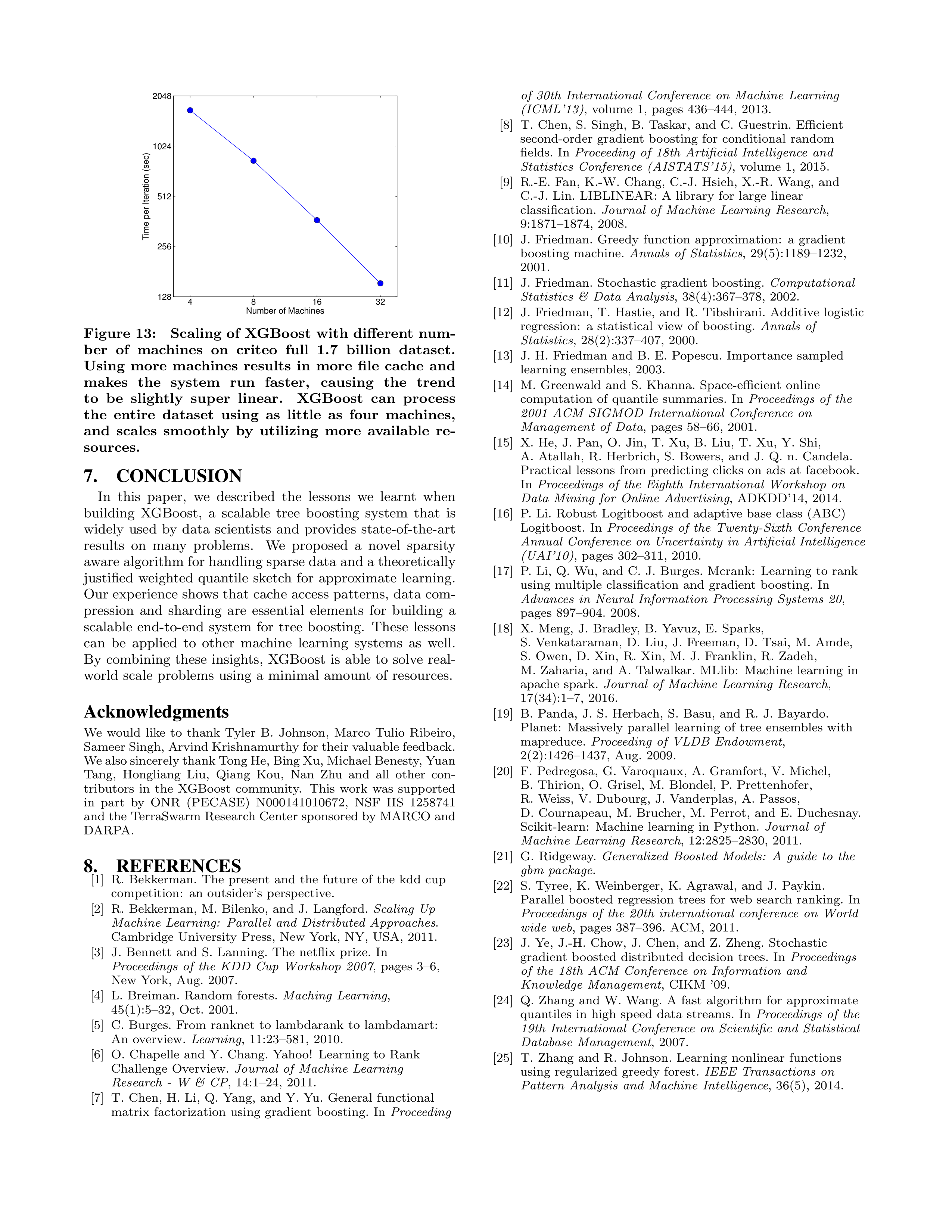
4
8
16
32
Number of Machines
128
256
512
1024
2048
Time per Iteration (sec)
Figure
13:
Scaling
of
XGBoost
with
different
num-
ber
of
machines
on
criteo
full
1.7
billion
dataset.
Using
more
machines
results
in
more
file
cache
and
makes
the
system
run
faster,
causing
the
trend
to
be
slightly
super
linear.
XGBoost
can
process
the
entire
dataset
using
as
little
as
four
machines,
and
scales
smoothly
by
utilizing
more
available
re-
sources.
7.
CONCLUSION
In
this
paper,
we
described
the
lessons
we
learnt
when
building
XGBoost,
a
scalable
tree
boosting
system
that
is
widely
used
by
data
scientists
and
provides
state-of-the-art
results
on
many
problems.
We
proposed
a
novel
sparsity
aware algorithm for handling sparse data and a theoretically
justified
weighted
quantile
sketch
for
approximate
learning.
Our
experience
shows
that
cache
access
patterns,
data
com-
pression
and
sharding
are
essential
elements
for
building
a
scalable
end-to-end
system
for
tree
boosting.
These
lessons
can
be
applied
to
other
machine
learning
systems
as
well.
By
combining
these
insights,
XGBoost
is
able
to
solve
real-
world
scale
problems
using
a
minimal
amount
of
resources.
Acknowledgments
We
would
like
to
thank
Tyler
B.
Johnson,
Marco
Tulio
Ribeiro,
Sameer Singh, Arvind Krishnamurthy for their valuable feedback.
We also sincerely thank Tong He, Bing Xu, Michael Benesty, Yuan
Tang,
Hongliang
Liu,
Qiang
Kou,
Nan
Zhu
and
all
other
con-
tributors
in
the
XGBoost
community.
This
work
was
supported
in
part
by
ONR
(PECASE)
N000141010672,
NSF
IIS
1258741
and the TerraSwarm Research Center sponsored by MARCO and
DARPA.
8.
REFERENCES
[1]
R.
Bekkerman.
The
present
and
the
future
of
the
kdd
cup
competition:
an
outsider’s
perspective.
[2]
R.
Bekkerman,
M.
Bilenko,
and
J.
Langford.
Scaling
Up
Machine
Learning:
Parallel
and
Distributed
Approaches
.
Cambridge
University
Press,
New
York,
NY,
USA,
2011.
[3]
J.
Bennett
and
S.
Lanning.
The
netflix
prize.
In
Proceedings
of
the
KDD
Cup
Workshop
2007
,
pages
3–6,
New
York,
Aug.
2007.
[4]
L.
Breiman.
Random
forests.
Maching
Learning
,
45(1):5–32,
Oct.
2001.
[5]
C.
Burges.
From
ranknet
to
lambdarank
to
lambdamart:
An
overview.
Learning
,
11:23–581,
2010.
[6]
O.
Chapelle
and
Y.
Chang.
Yahoo!
Learning
to
Rank
Challenge
Overview.
Journal
of
Machine
Learning
Research
-
W
&
CP
,
14:1–24,
2011.
[7]
T.
Chen,
H.
Li,
Q.
Yang,
and
Y.
Yu.
General
functional
matrix
factorization
using
gradient
boosting.
In
Proceeding
of
30th
International
Conference
on
Machine
Learning
(ICML’13)
,
volume
1,
pages
436–444,
2013.
[8]
T.
Chen,
S.
Singh,
B.
Taskar,
and
C.
Guestrin.
Efficient
second-order
gradient
boosting
for
conditional
random
fields.
In
Proceeding
of
18th
Artificial
Intelligence
and
Statistics
Conference
(AISTATS’15)
,
volume
1,
2015.
[9]
R.-E.
Fan,
K.-W.
Chang,
C.-J.
Hsieh,
X.-R.
Wang,
and
C.-J.
Lin.
LIBLINEAR:
A
library
for
large
linear
classification.
Journal
of
Machine
Learning
Research
,
9:1871–1874,
2008.
[10]
J.
Friedman.
Greedy
function
approximation:
a
gradient
boosting
machine.
Annals
of
Statistics
,
29(5):1189–1232,
2001.
[11]
J.
Friedman.
Stochastic
gradient
boosting.
Computational
Statistics
&
Data
Analysis
,
38(4):367–378,
2002.
[12]
J.
Friedman,
T.
Hastie,
and
R.
Tibshirani.
Additive
logistic
regression:
a
statistical
view
of
boosting.
Annals
of
Statistics
,
28(2):337–407,
2000.
[13]
J.
H.
Friedman
and
B.
E.
Popescu.
Importance
sampled
learning
ensembles,
2003.
[14]
M.
Greenwald
and
S.
Khanna.
Space-efficient
online
computation
of
quantile
summaries.
In
Proceedings
of
the
2001
ACM
SIGMOD
International
Conference
on
Management
of
Data
,
pages
58–66,
2001.
[15]
X.
He,
J.
Pan,
O.
Jin,
T.
Xu,
B.
Liu,
T.
Xu,
Y.
Shi,
A.
Atallah,
R.
Herbrich,
S.
Bowers,
and
J.
Q.
n.
Candela.
Practical
lessons
from
predicting
clicks
on
ads
at
facebook.
In
Proceedings
of
the
Eighth
International
Workshop
on
Data
Mining
for
Online
Advertising
,
ADKDD’14,
2014.
[16]
P.
Li.
Robust
Logitboost
and
adaptive
base
class
(ABC)
Logitboost.
In
Proceedings
of
the
Twenty-Sixth
Conference
Annual
Conference
on
Uncertainty
in
Artificial
Intelligence
(UAI’10)
,
pages
302–311,
2010.
[17]
P.
Li,
Q.
Wu,
and
C.
J.
Burges.
Mcrank:
Learning
to
rank
using
multiple
classification
and
gradient
boosting.
In
Advances
in
Neural
Information
Processing
Systems
20
,
pages
897–904.
2008.
[18]
X.
Meng,
J.
Bradley,
B.
Yavuz,
E.
Sparks,
S.
Venkataraman,
D.
Liu,
J.
Freeman,
D.
Tsai,
M.
Amde,
S.
Owen,
D.
Xin,
R.
Xin,
M.
J.
Franklin,
R.
Zadeh,
M.
Zaharia,
and
A.
Talwalkar.
MLlib:
Machine
learning
in
apache
spark.
Journal
of
Machine
Learning
Research
,
17(34):1–7,
2016.
[19]
B.
Panda,
J.
S.
Herbach,
S.
Basu,
and
R.
J.
Bayardo.
Planet:
Massively
parallel
learning
of
tree
ensembles
with
mapreduce.
Proceeding
of
VLDB
Endowment
,
2(2):1426–1437,
Aug.
2009.
[20]
F.
Pedregosa,
G.
Varoquaux,
A.
Gramfort,
V.
Michel,
B.
Thirion,
O.
Grisel,
M.
Blondel,
P.
Prettenhofer,
R.
Weiss,
V.
Dubourg,
J.
Vanderplas,
A.
Passos,
D.
Cournapeau,
M.
Brucher,
M.
Perrot,
and
E.
Duchesnay.
Scikit-learn:
Machine
learning
in
Python.
Journal
of
Machine
Learning
Research
,
12:2825–2830,
2011.
[21]
G.
Ridgeway.
Generalized
Boosted
Models:
A
guide
to
the
gbm
package
.
[22]
S.
Tyree,
K.
Weinberger,
K.
Agrawal,
and
J.
Paykin.
Parallel
boosted
regression
trees
for
web
search
ranking.
In
Proceedings
of
the
20th
international
conference
on
World
wide
web
,
pages
387–396.
ACM,
2011.
[23]
J.
Ye,
J.-H.
Chow,
J.
Chen,
and
Z.
Zheng.
Stochastic
gradient
boosted
distributed
decision
trees.
In
Proceedings
of
the
18th
ACM
Conference
on
Information
and
Knowledge
Management
,
CIKM
’09.
[24]
Q.
Zhang
and
W.
Wang.
A
fast
algorithm
for
approximate
quantiles
in
high
speed
data
streams.
In
Proceedings
of
the
19th
International
Conference
on
Scientific
and
Statistical
Database
Management
,
2007.
[25]
T.
Zhang
and
R.
Johnson.
Learning
nonlinear
functions
using
regularized
greedy
forest.
IEEE
Transactions
on
Pattern
Analysis
and
Machine
Intelligence
,
36(5),
2014.
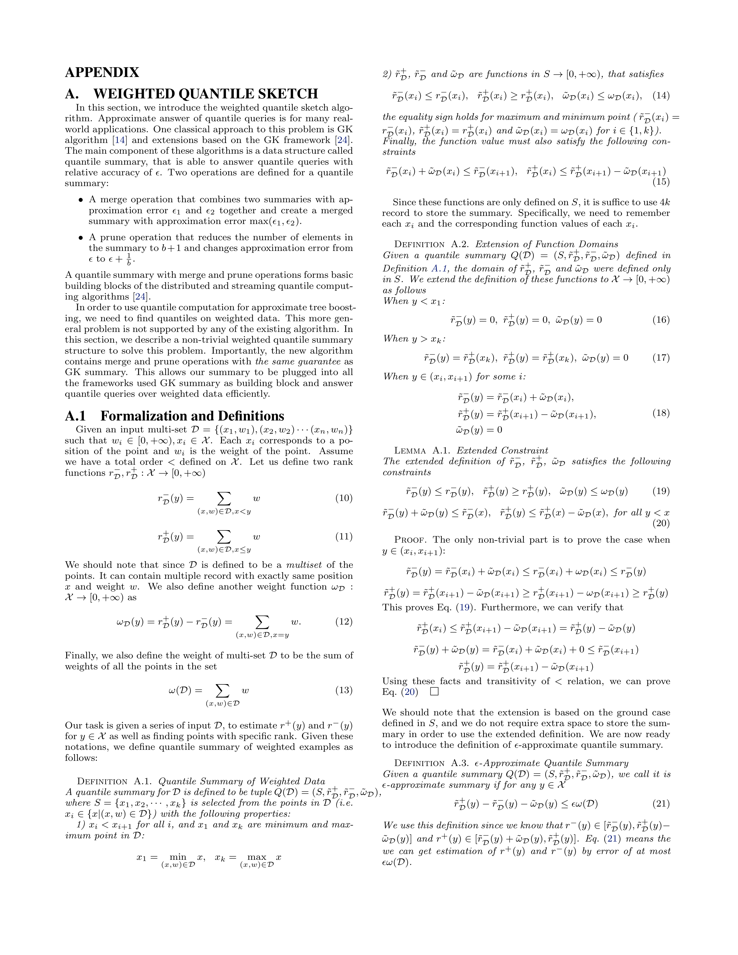
APPENDIX
A.
WEIGHTED QUANTILE SKETCH
In
this
section,
we
introduce
the
weighted
quantile
sketch
algo-
rithm.
Approximate
answer
of
quantile
queries
is
for
many
real-
world
applications.
One
classical
approach
to
this
problem
is
GK
algorithm
[
14
]
and
extensions
based
on
the
GK
framework
[
24
].
The main component of these algorithms is a data structure called
quantile
summary,
that
is
able
to
answer
quantile
queries
with
relative
accuracy
of
ϵ
.
Two
operations
are
defined
for
a
quantile
summary:
•
A
merge
operation
that
combines
two
summaries
with
ap-
proximation
error
ϵ
1
and
ϵ
2
together
and
create
a
merged
summary
with
approximation
error
max(
ϵ
1
, ϵ
2
).
•
A
prune
operation
that
reduces
the
number
of
elements
in
the summary to
b
+1 and changes approximation error from
ϵ
to
ϵ
+
1
b
.
A quantile summary with merge and prune operations forms basic
building blocks of the distributed and streaming quantile comput-
ing
algorithms
[
24
].
In order to use quantile computation for approximate tree boost-
ing,
we
need
to
find
quantiles
on
weighted
data.
This
more
gen-
eral problem is not supported by any of the existing algorithm.
In
this section,
we describe a non-trivial weighted quantile summary
structure
to
solve
this
problem.
Importantly,
the
new
algorithm
contains
merge
and
prune
operations
with
the
same
guarantee
as
GK
summary.
This
allows
our
summary
to
be
plugged
into
all
the
frameworks
used
GK
summary
as
building
block
and
answer
quantile
queries
over
weighted
data
efficiently.
A.1
Formalization and Definitions
Given
an
input
multi-set
D
=
{
(
x
1
, w
1
)
,
(
x
2
, w
2
)
· · ·
(
x
n
, w
n
)
}
such
that
w
i
∈
[0
,
+
∞
)
, x
i
∈X
.
Each
x
i
corresponds
to
a
po-
sition
of
the
point
and
w
i
is
the
weight
of
the
point.
Assume
we
have
a
total
order
<
defined
on
X
.
Let
us
define
two
rank
functions
r
−
D
, r
+
D
:
X
→
[0
,
+
∞
)
r
−
D
(
y
) =
X
(
x,w
)
∈D
,x<y
w
(10)
r
+
D
(
y
) =
X
(
x,w
)
∈D
,x
≤
y
w
(11)
We
should
note
that
since
D
is
defined
to
be
a
multiset
of
the
points.
It
can
contain
multiple
record
with
exactly
same
position
x
and
weight
w
.
We
also
define
another
weight
function
ω
D
:
X
→
[0
,
+
∞
)
as
ω
D
(
y
) =
r
+
D
(
y
)
−
r
−
D
(
y
) =
X
(
x,w
)
∈D
,x
=
y
w.
(12)
Finally,
we
also
define
the
weight
of
multi-set
D
to
be
the
sum
of
weights
of
all
the
points
in
the
set
ω
(
D
) =
X
(
x,w
)
∈D
w
(13)
Our task is given a series of input
D
, to estimate
r
+
(
y
) and
r
−
(
y
)
for
y
∈X
as well as finding points with specific rank.
Given these
notations,
we
define
quantile
summary
of
weighted
examples
as
follows:
Definition
A.1.
Quantile
Summary
of
Weighted
Data
A quantile summary for
D
is defined to be tuple
Q
(
D
) = (
S,
˜
r
+
D
,
˜
r
−
D
,
˜
ω
D
)
,
where
S
=
{
x
1
, x
2
,
· · ·
, x
k
}
is
selected
from
the
points
in
D
(i.e.
x
i
∈{
x
|
(
x, w
)
∈D}
)
with
the
following
properties:
1)
x
i
< x
i
+1
for
all
i
,
and
x
1
and
x
k
are
minimum
and
max-
imum
point
in
D
:
x
1
=
min
(
x,w
)
∈D
x,
x
k
=
max
(
x,w
)
∈D
x
2)
˜
r
+
D
,
˜
r
−
D
and
˜
ω
D
are
functions
in
S
→
[0
,
+
∞
)
,
that
satisfies
˜
r
−
D
(
x
i
)
≤
r
−
D
(
x
i
)
,
˜
r
+
D
(
x
i
)
≥
r
+
D
(
x
i
)
,
˜
ω
D
(
x
i
)
≤
ω
D
(
x
i
)
,
(14)
the equality sign holds for maximum and minimum point (
˜
r
−
D
(
x
i
) =
r
−
D
(
x
i
)
,
˜
r
+
D
(
x
i
) =
r
+
D
(
x
i
)
and
˜
ω
D
(
x
i
) =
ω
D
(
x
i
)
for
i
∈{
1
, k
}
).
Finally,
the
function
value
must
also
satisfy
the
following
con-
straints
˜
r
−
D
(
x
i
) +
˜
ω
D
(
x
i
)
≤
˜
r
−
D
(
x
i
+1
)
,
˜
r
+
D
(
x
i
)
≤
˜
r
+
D
(
x
i
+1
)
−
˜
ω
D
(
x
i
+1
)
(15)
Since these functions are only defined on
S
, it is suffice to use 4
k
record
to
store
the
summary.
Specifically,
we
need
to
remember
each
x
i
and
the
corresponding
function
values
of
each
x
i
.
Definition
A.2.
Extension
of
Function
Domains
Given
a
quantile
summary
Q
(
D
)
=
(
S,
˜
r
+
D
,
˜
r
−
D
,
˜
ω
D
)
defined
in
Definition
A.1
,
the
domain
of
˜
r
+
D
,
˜
r
−
D
and
˜
ω
D
were
defined
only
in
S
.
We extend the definition of these functions to
X
→
[0
,
+
∞
)
as
follows
When
y
< x
1
:
˜
r
−
D
(
y
) = 0
,
˜
r
+
D
(
y
) = 0
,
˜
ω
D
(
y
) = 0
(16)
When
y
> x
k
:
˜
r
−
D
(
y
) =
˜
r
+
D
(
x
k
)
,
˜
r
+
D
(
y
) =
˜
r
+
D
(
x
k
)
,
˜
ω
D
(
y
) = 0
(17)
When
y
∈
(
x
i
, x
i
+1
)
for
some
i
:
˜
r
−
D
(
y
) =
˜
r
−
D
(
x
i
) +
˜
ω
D
(
x
i
)
,
˜
r
+
D
(
y
) =
˜
r
+
D
(
x
i
+1
)
−
˜
ω
D
(
x
i
+1
)
,
˜
ω
D
(
y
) = 0
(18)
Lemma
A.1.
Extended
Constraint
The
extended
definition
of
˜
r
−
D
,
˜
r
+
D
,
˜
ω
D
satisfies
the
following
constraints
˜
r
−
D
(
y
)
≤
r
−
D
(
y
)
,
˜
r
+
D
(
y
)
≥
r
+
D
(
y
)
,
˜
ω
D
(
y
)
≤
ω
D
(
y
)
(19)
˜
r
−
D
(
y
) +
˜
ω
D
(
y
)
≤
˜
r
−
D
(
x
)
,
˜
r
+
D
(
y
)
≤
˜
r
+
D
(
x
)
−
˜
ω
D
(
x
)
,
for
all
y
< x
(20)
Proof.
The
only
non-trivial
part
is
to
prove
the
case
when
y
∈
(
x
i
, x
i
+1
):
˜
r
−
D
(
y
) =
˜
r
−
D
(
x
i
) +
˜
ω
D
(
x
i
)
≤
r
−
D
(
x
i
) +
ω
D
(
x
i
)
≤
r
−
D
(
y
)
˜
r
+
D
(
y
) =
˜
r
+
D
(
x
i
+1
)
−
˜
ω
D
(
x
i
+1
)
≥
r
+
D
(
x
i
+1
)
−
ω
D
(
x
i
+1
)
≥
r
+
D
(
y
)
This
proves
Eq.
(
19
).
Furthermore,
we
can
verify
that
˜
r
+
D
(
x
i
)
≤
˜
r
+
D
(
x
i
+1
)
−
˜
ω
D
(
x
i
+1
) =
˜
r
+
D
(
y
)
−
˜
ω
D
(
y
)
˜
r
−
D
(
y
) +
˜
ω
D
(
y
) =
˜
r
−
D
(
x
i
) +
˜
ω
D
(
x
i
) + 0
≤
˜
r
−
D
(
x
i
+1
)
˜
r
+
D
(
y
) =
˜
r
+
D
(
x
i
+1
)
−
˜
ω
D
(
x
i
+1
)
Using
these
facts
and
transitivity
of
<
relation,
we
can
prove
Eq.
(
20
)
We
should
note
that
the
extension
is
based
on
the
ground
case
defined
in
S
,
and
we
do
not
require
extra
space
to
store
the
sum-
mary
in
order
to
use
the
extended
definition.
We
are
now
ready
to
introduce
the
definition
of
ϵ
-approximate
quantile
summary.
Definition
A.3.
ϵ
-Approximate
Quantile
Summary
Given
a
quantile
summary
Q
(
D
)
=
(
S,
˜
r
+
D
,
˜
r
−
D
,
˜
ω
D
)
,
we
call
it
is
ϵ
-approximate
summary
if
for
any
y
∈X
˜
r
+
D
(
y
)
−
˜
r
−
D
(
y
)
−
˜
ω
D
(
y
)
≤
ϵω
(
D
)
(21)
We use this definition since we know that
r
−
(
y
)
∈
[˜
r
−
D
(
y
)
,
˜
r
+
D
(
y
)
−
˜
ω
D
(
y
)]
and
r
+
(
y
)
∈
[˜
r
−
D
(
y
) +
˜
ω
D
(
y
)
,
˜
r
+
D
(
y
)]
.
Eq.
(
21
)
means
the
we
can
get
estimation
of
r
+
(
y
)
and
r
−
(
y
)
by
error
of
at
most
ϵω
(
D
)
.
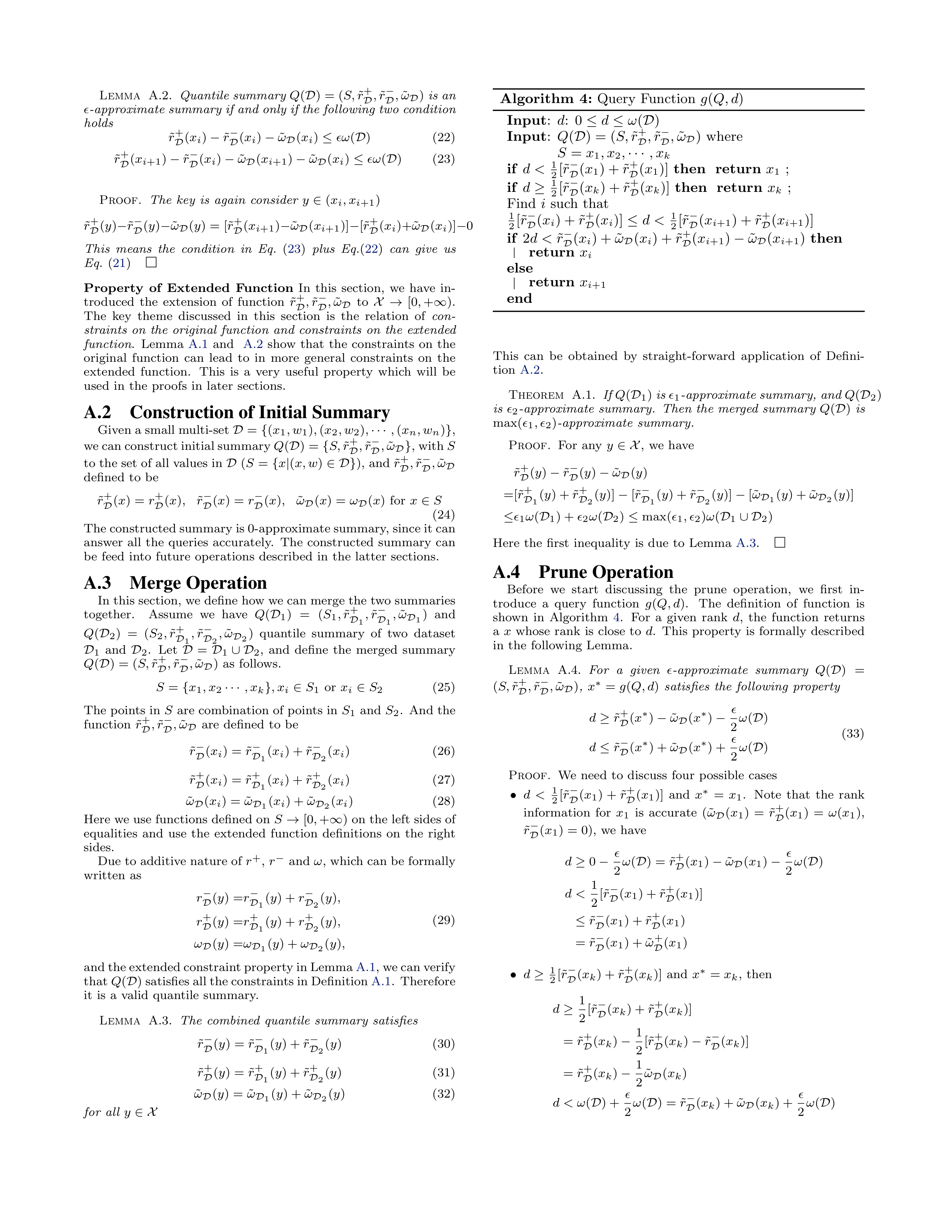
Lemma
A.2.
Quantile
summary
Q
(
D
) = (
S,
˜
r
+
D
,
˜
r
−
D
,
˜
ω
D
)
is
an
ϵ
-approximate
summary
if
and
only
if
the
following
two
condition
holds
˜
r
+
D
(
x
i
)
−
˜
r
−
D
(
x
i
)
−
˜
ω
D
(
x
i
)
≤
ϵω
(
D
)
(22)
˜
r
+
D
(
x
i
+1
)
−
˜
r
−
D
(
x
i
)
−
˜
ω
D
(
x
i
+1
)
−
˜
ω
D
(
x
i
)
≤
ϵω
(
D
)
(23)
Proof.
The
key
is
again
consider
y
∈
(
x
i
, x
i
+1
)
˜
r
+
D
(
y
)
−
˜
r
−
D
(
y
)
−
˜
ω
D
(
y
) = [˜
r
+
D
(
x
i
+1
)
−
˜
ω
D
(
x
i
+1
)]
−
[˜
r
+
D
(
x
i
)+˜
ω
D
(
x
i
)]
−
0
This
means
the
condition
in
Eq.
(
23
)
plus
Eq.
(
22
)
can
give
us
Eq.
(
21
)
Property
of
Extended
Function
In
this
section,
we
have
in-
troduced
the
extension
of
function
˜
r
+
D
,
˜
r
−
D
,
˜
ω
D
to
X
→
[0
,
+
∞
).
The
key
theme
discussed
in
this
section
is
the
relation
of
con-
straints
on
the
original
function
and
constraints
on
the
extended
function
.
Lemma
A.1
and
A.2
show
that
the
constraints
on
the
original
function
can
lead
to
in
more
general
constraints
on
the
extended
function.
This
is
a
very
useful
property
which
will
be
used
in
the
proofs
in
later
sections.
A.2
Construction of Initial Summary
Given a small multi-set
D
=
{
(
x
1
, w
1
)
,
(
x
2
, w
2
)
,
· · ·
,
(
x
n
, w
n
)
}
,
we can construct initial summary
Q
(
D
) =
{
S,
˜
r
+
D
,
˜
r
−
D
,
˜
ω
D
}
, with
S
to
the
set
of all
values
in
D
(
S
=
{
x
|
(
x, w
)
∈D}
),
and
˜
r
+
D
,
˜
r
−
D
,
˜
ω
D
defined
to
be
˜
r
+
D
(
x
) =
r
+
D
(
x
)
,
˜
r
−
D
(
x
) =
r
−
D
(
x
)
,
˜
ω
D
(
x
) =
ω
D
(
x
)
for
x
∈
S
(24)
The constructed summary is 0-approximate summary, since it can
answer
all
the
queries
accurately.
The
constructed
summary
can
be
feed
into
future
operations
described
in
the
latter
sections.
A.3
Merge Operation
In this section,
we define how we can merge the two summaries
together.
Assume
we
have
Q
(
D
1
)
=
(
S
1
,
˜
r
+
D
1
,
˜
r
−
D
1
,
˜
ω
D
1
)
and
Q
(
D
2
)
=
(
S
2
,
˜
r
+
D
1
,
˜
r
−
D
2
,
˜
ω
D
2
)
quantile
summary
of
two
dataset
D
1
and
D
2
.
Let
D
=
D
1
∪D
2
,
and
define
the
merged
summary
Q
(
D
) = (
S,
˜
r
+
D
,
˜
r
−
D
,
˜
ω
D
)
as
follows.
S
=
{
x
1
, x
2
· · ·
, x
k
}
, x
i
∈
S
1
or
x
i
∈
S
2
(25)
The
points
in
S
are
combination
of
points
in
S
1
and
S
2
.
And
the
function
˜
r
+
D
,
˜
r
−
D
,
˜
ω
D
are
defined
to
be
˜
r
−
D
(
x
i
) =
˜
r
−
D
1
(
x
i
) + ˜
r
−
D
2
(
x
i
)
(26)
˜
r
+
D
(
x
i
) =
˜
r
+
D
1
(
x
i
) + ˜
r
+
D
2
(
x
i
)
(27)
˜
ω
D
(
x
i
) =
˜
ω
D
1
(
x
i
) +
˜
ω
D
2
(
x
i
)
(28)
Here
we
use
functions
defined
on
S
→
[0
,
+
∞
)
on
the
left
sides
of
equalities
and
use
the
extended
function
definitions
on
the
right
sides.
Due
to
additive
nature
of
r
+
,
r
−
and
ω
,
which
can
be
formally
written
as
r
−
D
(
y
) =
r
−
D
1
(
y
) +
r
−
D
2
(
y
)
,
r
+
D
(
y
) =
r
+
D
1
(
y
) +
r
+
D
2
(
y
)
,
ω
D
(
y
) =
ω
D
1
(
y
) +
ω
D
2
(
y
)
,
(29)
and the extended constraint property in Lemma
A.1
, we can verify
that
Q
(
D
) satisfies all the constraints in Definition
A.1
.
Therefore
it
is
a
valid
quantile
summary.
Lemma
A.3.
The
combined
quantile
summary
satisfies
˜
r
−
D
(
y
) =
˜
r
−
D
1
(
y
) + ˜
r
−
D
2
(
y
)
(30)
˜
r
+
D
(
y
) =
˜
r
+
D
1
(
y
) + ˜
r
+
D
2
(
y
)
(31)
˜
ω
D
(
y
) =
˜
ω
D
1
(
y
) +
˜
ω
D
2
(
y
)
(32)
for
all
y
∈X
Algorithm
4:
Query
Function
g
(
Q, d
)
Input
:
d
:
0
≤
d
≤
ω
(
D
)
Input
:
Q
(
D
) = (
S,
˜
r
+
D
,
˜
r
−
D
,
˜
ω
D
)
where
S
=
x
1
, x
2
,
· · ·
, x
k
if
d <
1
2
[˜
r
−
D
(
x
1
) + ˜
r
+
D
(
x
1
)]
then
return
x
1
;
if
d
≥
1
2
[˜
r
−
D
(
x
k
) + ˜
r
+
D
(
x
k
)]
then
return
x
k
;
Find
i
such
that
1
2
[˜
r
−
D
(
x
i
) + ˜
r
+
D
(
x
i
)]
≤
d <
1
2
[˜
r
−
D
(
x
i
+1
) + ˜
r
+
D
(
x
i
+1
)]
if
2
d <
˜
r
−
D
(
x
i
) +
˜
ω
D
(
x
i
) + ˜
r
+
D
(
x
i
+1
)
−
˜
ω
D
(
x
i
+1
)
then
return
x
i
else
return
x
i
+1
end
This
can
be
obtained
by
straight-forward
application
of
Defini-
tion
A.2
.
Theorem
A.1.
If
Q
(
D
1
)
is
ϵ
1
-approximate summary, and
Q
(
D
2
)
is
ϵ
2
-approximate
summary.
Then
the
merged
summary
Q
(
D
)
is
max(
ϵ
1
, ϵ
2
)
-approximate
summary.
Proof.
For
any
y
∈X
,
we
have
˜
r
+
D
(
y
)
−
˜
r
−
D
(
y
)
−
˜
ω
D
(
y
)
=[˜
r
+
D
1
(
y
) + ˜
r
+
D
2
(
y
)]
−
[˜
r
−
D
1
(
y
) + ˜
r
−
D
2
(
y
)]
−
[˜
ω
D
1
(
y
) +
˜
ω
D
2
(
y
)]
≤
ϵ
1
ω
(
D
1
) +
ϵ
2
ω
(
D
2
)
≤
max(
ϵ
1
, ϵ
2
)
ω
(
D
1
∪D
2
)
Here
the
first
inequality
is
due
to
Lemma
A.3
.
A.4
Prune Operation
Before
we
start
discussing
the
prune
operation,
we
first
in-
troduce
a
query
function
g
(
Q, d
).
The
definition
of
function
is
shown
in
Algorithm
4
.
For
a
given
rank
d
,
the
function
returns
a
x
whose
rank
is
close
to
d
.
This
property
is
formally
described
in
the
following
Lemma.
Lemma
A.4.
For
a
given
ϵ
-approximate
summary
Q
(
D
)
=
(
S,
˜
r
+
D
,
˜
r
−
D
,
˜
ω
D
)
,
x
∗
=
g
(
Q, d
)
satisfies
the
following
property
d
≥
˜
r
+
D
(
x
∗
)
−
˜
ω
D
(
x
∗
)
−
ϵ
2
ω
(
D
)
d
≤
˜
r
−
D
(
x
∗
) +
˜
ω
D
(
x
∗
) +
ϵ
2
ω
(
D
)
(33)
Proof.
We
need
to
discuss
four
possible
cases
•
d
<
1
2
[˜
r
−
D
(
x
1
) +
˜
r
+
D
(
x
1
)]
and
x
∗
=
x
1
.
Note
that
the
rank
information
for
x
1
is
accurate
(˜
ω
D
(
x
1
)
=
˜
r
+
D
(
x
1
)
=
ω
(
x
1
),
˜
r
−
D
(
x
1
) = 0),
we
have
d
≥
0
−
ϵ
2
ω
(
D
) =
˜
r
+
D
(
x
1
)
−
˜
ω
D
(
x
1
)
−
ϵ
2
ω
(
D
)
d <
1
2
[˜
r
−
D
(
x
1
) + ˜
r
+
D
(
x
1
)]
≤
˜
r
−
D
(
x
1
) + ˜
r
+
D
(
x
1
)
=
˜
r
−
D
(
x
1
) +
˜
ω
+
D
(
x
1
)
•
d
≥
1
2
[˜
r
−
D
(
x
k
) + ˜
r
+
D
(
x
k
)]
and
x
∗
=
x
k
,
then
d
≥
1
2
[˜
r
−
D
(
x
k
) + ˜
r
+
D
(
x
k
)]
=
˜
r
+
D
(
x
k
)
−
1
2
[˜
r
+
D
(
x
k
)
−
˜
r
−
D
(
x
k
)]
=
˜
r
+
D
(
x
k
)
−
1
2
˜
ω
D
(
x
k
)
d < ω
(
D
) +
ϵ
2
ω
(
D
) =
˜
r
−
D
(
x
k
) +
˜
ω
D
(
x
k
) +
ϵ
2
ω
(
D
)
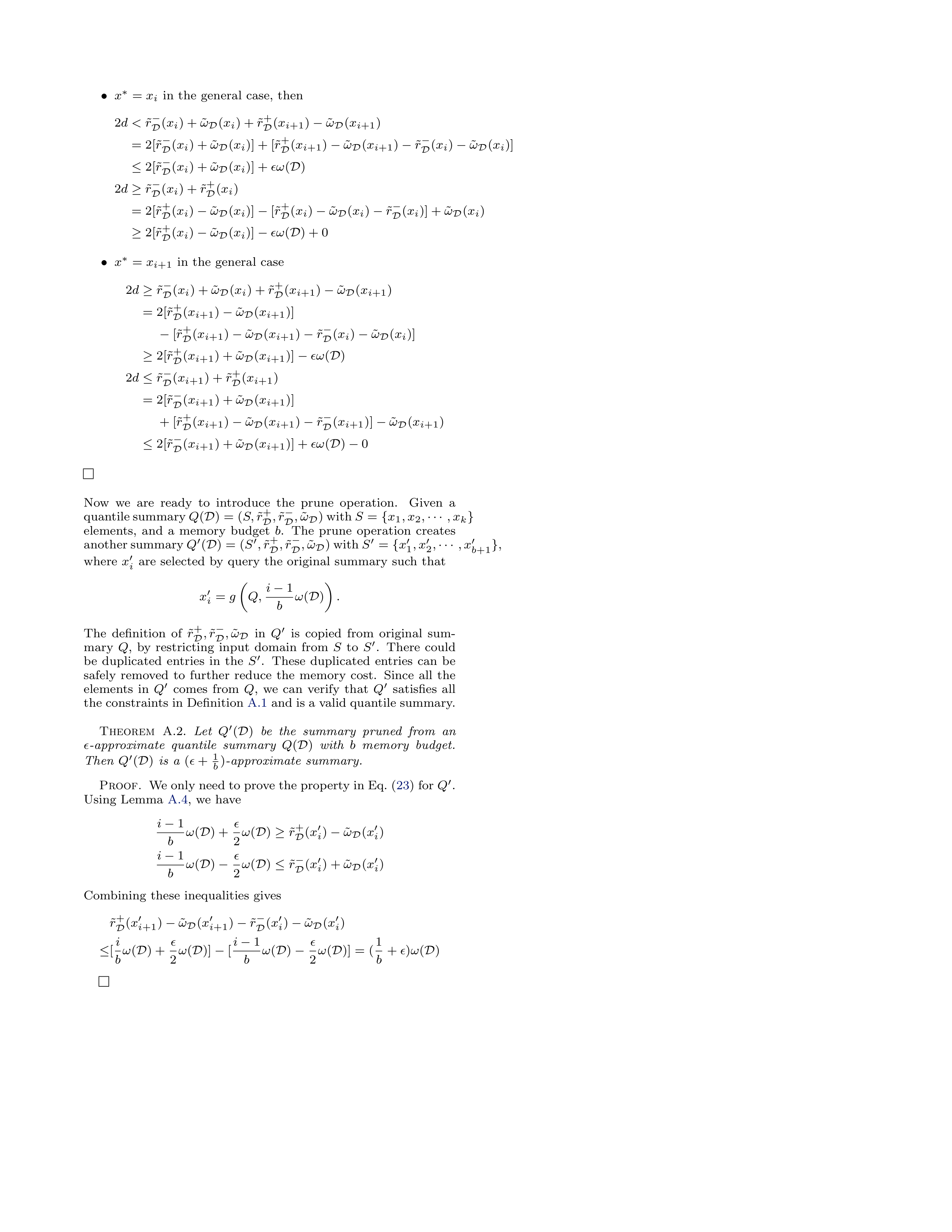
•
x
∗
=
x
i
in
the
general
case,
then
2
d <
˜
r
−
D
(
x
i
) +
˜
ω
D
(
x
i
) + ˜
r
+
D
(
x
i
+1
)
−
˜
ω
D
(
x
i
+1
)
= 2[˜
r
−
D
(
x
i
) +
˜
ω
D
(
x
i
)] + [˜
r
+
D
(
x
i
+1
)
−
˜
ω
D
(
x
i
+1
)
−
˜
r
−
D
(
x
i
)
−
˜
ω
D
(
x
i
)]
≤
2[˜
r
−
D
(
x
i
) +
˜
ω
D
(
x
i
)] +
ϵω
(
D
)
2
d
≥
˜
r
−
D
(
x
i
) + ˜
r
+
D
(
x
i
)
= 2[˜
r
+
D
(
x
i
)
−
˜
ω
D
(
x
i
)]
−
[˜
r
+
D
(
x
i
)
−
˜
ω
D
(
x
i
)
−
˜
r
−
D
(
x
i
)] +
˜
ω
D
(
x
i
)
≥
2[˜
r
+
D
(
x
i
)
−
˜
ω
D
(
x
i
)]
−
ϵω
(
D
) + 0
•
x
∗
=
x
i
+1
in
the
general
case
2
d
≥
˜
r
−
D
(
x
i
) +
˜
ω
D
(
x
i
) + ˜
r
+
D
(
x
i
+1
)
−
˜
ω
D
(
x
i
+1
)
= 2[˜
r
+
D
(
x
i
+1
)
−
˜
ω
D
(
x
i
+1
)]
−
[˜
r
+
D
(
x
i
+1
)
−
˜
ω
D
(
x
i
+1
)
−
˜
r
−
D
(
x
i
)
−
˜
ω
D
(
x
i
)]
≥
2[˜
r
+
D
(
x
i
+1
) +
˜
ω
D
(
x
i
+1
)]
−
ϵω
(
D
)
2
d
≤
˜
r
−
D
(
x
i
+1
) + ˜
r
+
D
(
x
i
+1
)
= 2[˜
r
−
D
(
x
i
+1
) +
˜
ω
D
(
x
i
+1
)]
+ [˜
r
+
D
(
x
i
+1
)
−
˜
ω
D
(
x
i
+1
)
−
˜
r
−
D
(
x
i
+1
)]
−
˜
ω
D
(
x
i
+1
)
≤
2[˜
r
−
D
(
x
i
+1
) +
˜
ω
D
(
x
i
+1
)] +
ϵω
(
D
)
−
0
Now
we
are
ready
to
introduce
the
prune
operation.
Given
a
quantile summary
Q
(
D
) = (
S,
˜
r
+
D
,
˜
r
−
D
,
˜
ω
D
) with
S
=
{
x
1
, x
2
,
· · ·
, x
k
}
elements,
and
a
memory
budget
b
.
The
prune
operation
creates
another summary
Q
′
(
D
) = (
S
′
,
˜
r
+
D
,
˜
r
−
D
,
˜
ω
D
) with
S
′
=
{
x
′
1
, x
′
2
,
· · ·
, x
′
b
+1
}
,
where
x
′
i
are
selected
by
query
the
original
summary
such
that
x
′
i
=
g
Q,
i
−
1
b
ω
(
D
)
.
The
definition
of
˜
r
+
D
,
˜
r
−
D
,
˜
ω
D
in
Q
′
is
copied
from
original
sum-
mary
Q
,
by
restricting
input
domain
from
S
to
S
′
.
There
could
be
duplicated
entries
in
the
S
′
.
These
duplicated
entries
can
be
safely
removed
to
further
reduce
the
memory
cost.
Since
all
the
elements
in
Q
′
comes
from
Q
,
we
can
verify
that
Q
′
satisfies
all
the constraints in Definition
A.1
and is
a
valid
quantile summary.
Theorem
A.2.
Let
Q
′
(
D
)
be
the
summary
pruned
from
an
ϵ
-approximate
quantile
summary
Q
(
D
)
with
b
memory
budget.
Then
Q
′
(
D
)
is
a
(
ϵ
+
1
b
)
-approximate
summary.
Proof.
We only need to prove the property in Eq. (
23
) for
Q
′
.
Using
Lemma
A.4
,
we
have
i
−
1
b
ω
(
D
) +
ϵ
2
ω
(
D
)
≥
˜
r
+
D
(
x
′
i
)
−
˜
ω
D
(
x
′
i
)
i
−
1
b
ω
(
D
)
−
ϵ
2
ω
(
D
)
≤
˜
r
−
D
(
x
′
i
) +
˜
ω
D
(
x
′
i
)
Combining
these
inequalities
gives
˜
r
+
D
(
x
′
i
+1
)
−
˜
ω
D
(
x
′
i
+1
)
−
˜
r
−
D
(
x
′
i
)
−
˜
ω
D
(
x
′
i
)
≤
[
i
b
ω
(
D
) +
ϵ
2
ω
(
D
)]
−
[
i
−
1
b
ω
(
D
)
−
ϵ
2
ω
(
D
)] = ( 1
b
+
ϵ
)
ω
(
D
)