SPEECH RECOGNITION WITH DEEP RECURRENT NEURAL NETWORKS
Alex Graves, Abdel-rahman Mohamed and Geoffrey Hinton
Department of Computer Science, University of Toronto
ABSTRACT
Recurrent neural networks (RNNs) are a powerful model for
sequential data. End-to-end training methods such as Connec-
tionist Temporal Classification make it possible to train RNNs
for sequence labelling problems where the input-output align-
ment
is
unknown.
The
combination
of
these
methods
with
the
Long
Short-term
Memory
RNN
architecture
has
proved
particularly
fruitful,
delivering
state-of-the-art
results
in
cur-
sive handwriting recognition.
However RNN performance in
speech recognition has so far been disappointing, with better
results returned by deep feedforward networks. This paper in-
vestigates
deep recurrent neural networks
, which combine the
multiple levels of representation that have proved so effective
in
deep
networks
with
the
flexible
use
of
long
range
context
that
empowers
RNNs.
When
trained
end-to-end
with
suit-
able regularisation, we find that deep Long Short-term Mem-
ory
RNNs
achieve
a
test
set
error
of
17.7%
on
the
TIMIT
phoneme recognition benchmark, which to our knowledge is
the best recorded score.
Index
Terms
—
recurrent
neural
networks,
deep
neural
networks, speech recognition
1.
INTRODUCTION
Neural
networks
have
a
long
history
in
speech
recognition,
usually
in
combination
with
hidden
Markov
models
[1,
2].
They have gained attention in recent years with the dramatic
improvements
in
acoustic
modelling
yielded
by
deep
feed-
forward
networks
[3,
4].
Given
that
speech
is
an
inherently
dynamic
process,
it
seems
natural
to
consider
recurrent
neu-
ral
networks
(RNNs)
as
an
alternative
model.
HMM-RNN
systems [5] have also seen
a recent revival
[6, 7],
but do not
currently perform as well as deep networks.
Instead
of
combining
RNNs
with
HMMs,
it
is
possible
to train RNNs ‘end-to-end’ for speech recognition [8, 9, 10].
This
approach
exploits
the
larger
state-space
and
richer
dy-
namics
of
RNNs
compared
to
HMMs,
and
avoids
the
prob-
lem
of
using
potentially
incorrect
alignments
as
training
tar-
gets.
The combination of Long Short-term Memory [11], an
RNN architecture with an improved memory, with end-to-end
training has proved especially effective for cursive handwrit-
ing
recognition
[12,
13].
However
it
has
so
far
made
little
impact on speech recognition.
RNNs are inherently deep in time, since their hidden state
is a function of all previous hidden states.
The question that
inspired this paper was whether RNNs could also benefit from
depth
in
space;
that
is
from
stacking
multiple
recurrent
hid-
den layers on top of each other, just as feedforward layers are
stacked in conventional deep networks.
To answer this ques-
tion
we
introduce
deep
Long
Short-term
Memory
RNNs
and
assess their potential for speech recognition.
We also present
an enhancement to a recently introduced end-to-end learning
method that jointly trains two separate RNNs as acoustic and
linguistic models [10].
Sections 2 and 3 describe the network
architectures and training methods, Section 4 provides exper-
imental results and concluding remarks are given in Section 5.
2.
RECURRENT NEURAL NETWORKS
Given an input sequence
x
= (
x
1
, . . . , x
T
)
, a standard recur-
rent
neural
network
(RNN)
computes
the
hidden
vector
se-
quence
h
=
(
h
1
, . . . , h
T
)
and
output
vector
sequence
y
=
(
y
1
, . . . , y
T
)
by iterating the following equations from
t
=
1
to
T
:
h
t
=
H
(
W
xh
x
t
+
W
hh
h
t
−
1
+
b
h
)
(1)
y
t
=
W
hy
h
t
+
b
y
(2)
where
the
W
terms
denote
weight
matrices
(e.g.
W
xh
is
the
input-hidden
weight
matrix),
the
b
terms
denote
bias vectors
(e.g.
b
h
is hidden bias vector) and
H
is the hidden layer func-
tion.
H
is
usually
an
elementwise
application
of
a
sigmoid
function.
However we have found that the Long Short-Term
Memory (LSTM) architecture [11], which uses purpose-built
memory cells
to store information, is better at finding and ex-
ploiting long range context.
Fig. 1 illustrates a single LSTM
memory cell. For the version of LSTM used in this paper [14]
H
is implemented by the following composite function:
i
t
=
σ
(
W
xi
x
t
+
W
hi
h
t
−
1
+
W
ci
c
t
−
1
+
b
i
)
(3)
f
t
=
σ
(
W
xf
x
t
+
W
hf
h
t
−
1
+
W
cf
c
t
−
1
+
b
f
)
(4)
c
t
=
f
t
c
t
−
1
+
i
t
tanh (
W
xc
x
t
+
W
hc
h
t
−
1
+
b
c
)
(5)
o
t
=
σ
(
W
xo
x
t
+
W
ho
h
t
−
1
+
W
co
c
t
+
b
o
)
(6)
h
t
=
o
t
tanh(
c
t
)
(7)
where
σ
is
the
logistic
sigmoid
function,
and
i
,
f
,
o
and
c
are
respectively
the
input
gate
,
forget
gate
,
output
gate
and
arXiv:1303.5778v1 [cs.NE] 22 Mar 2013
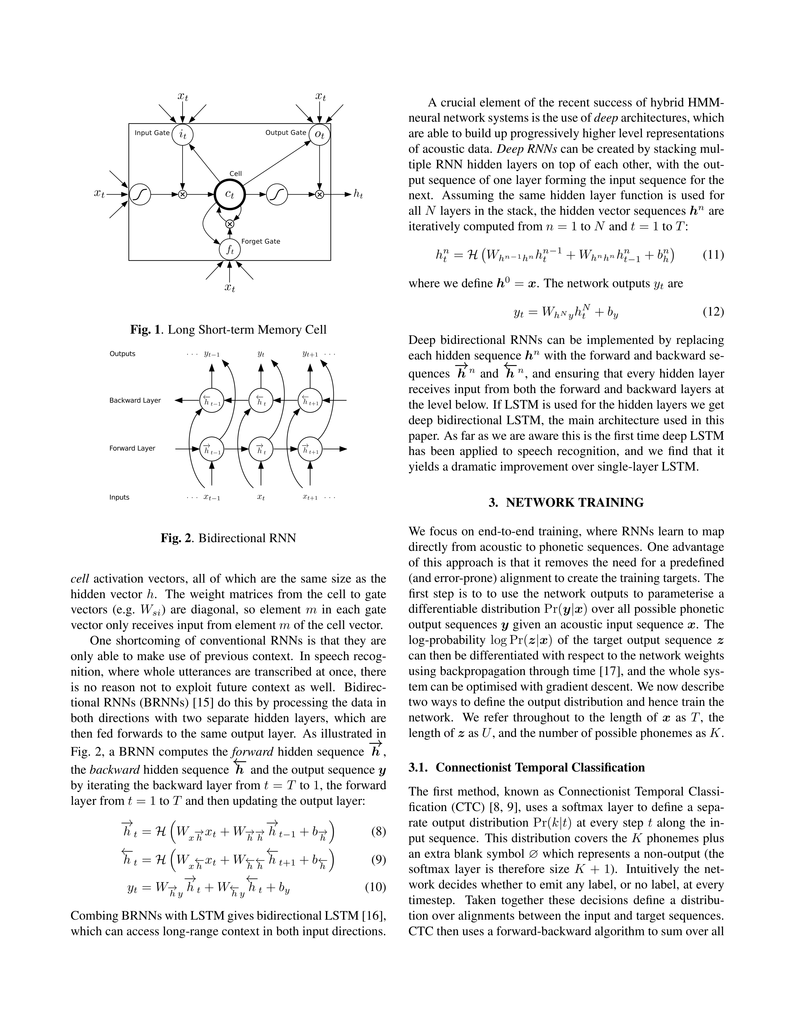
Fig. 1
.
Long Short-term Memory Cell
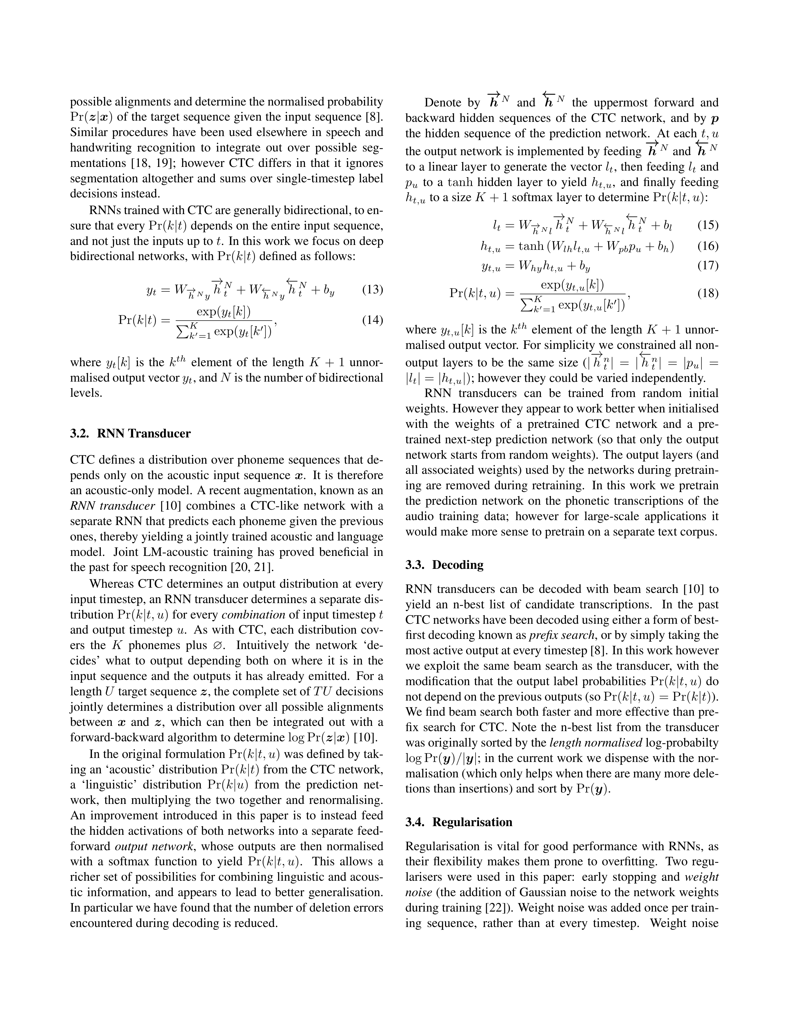
Fig. 2
.
Bidirectional RNN
cell
activation
vectors,
all
of
which
are
the
same
size
as
the
hidden
vector
h
.
The
weight
matrices
from
the
cell
to
gate
vectors
(e.g.
W
si
)
are
diagonal,
so
element
m
in
each
gate
vector only receives input from element
m
of the cell vector.
One
shortcoming
of
conventional
RNNs
is
that
they
are
only
able
to
make
use
of
previous
context.
In
speech
recog-
nition,
where whole utterances
are transcribed
at
once,
there
is
no
reason
not
to
exploit
future
context
as
well.
Bidirec-
tional RNNs (BRNNs) [15] do this by processing the data in
both
directions
with
two
separate
hidden
layers,
which
are
then
fed
forwards
to
the
same
output
layer.
As
illustrated
in
Fig.
2,
a
BRNN
computes
the
forward
hidden
sequence
−
→
h
,
the
backward
hidden sequence
←
−
h
and the output sequence
y
by iterating the backward layer from
t
=
T
to
1
, the forward
layer from
t
= 1
to
T
and then updating the output layer:
−→
h
t
=
H
W
x
−
→
h
x
t
+
W
−
→
h
−
→
h
−→
h
t
−
1
+
b
−
→
h
(8)
←−
h
t
=
H
W
x
←
−
h
x
t
+
W
←
−
h
←
−
h
←−
h
t
+1
+
b
←
−
h
(9)
y
t
=
W
−
→
h y
−→
h
t
+
W
←
−
h y
←−
h
t
+
b
y
(10)
Combing BRNNs with LSTM gives bidirectional LSTM [16],
which can access long-range context in both input directions.
A crucial element of the recent success of hybrid HMM-
neural network systems is the use of
deep
architectures, which
are able to build up progressively higher level representations
of acoustic data.
Deep RNNs
can be created by stacking mul-
tiple
RNN
hidden
layers
on
top
of
each
other,
with
the
out-
put sequence of one layer forming the input sequence for the
next.
Assuming
the
same
hidden
layer
function
is
used
for
all
N
layers in the stack, the hidden vector sequences
h
n
are
iteratively computed from
n
= 1
to
N
and
t
= 1
to
T
:
h
n
t
=
H
W
h
n
−
1
h
n
h
n
−
1
t
+
W
h
n
h
n
h
n
t
−
1
+
b
n
h
(11)
where we define
h
0
=
x
.
The network outputs
y
t
are
y
t
=
W
h
N
y
h
N
t
+
b
y
(12)
Deep
bidirectional
RNNs
can
be
implemented
by
replacing
each hidden sequence
h
n
with the forward and backward se-
quences
−
→
h
n
and
←
−
h
n
,
and
ensuring
that
every
hidden
layer
receives input from both the forward and backward layers at
the level below.
If LSTM is used for the hidden layers we get
deep
bidirectional
LSTM,
the
main
architecture
used
in
this
paper.
As far as we are aware this is the first time deep LSTM
has
been
applied
to
speech
recognition,
and
we
find
that
it
yields a dramatic improvement over single-layer LSTM.
3.
NETWORK TRAINING
We
focus
on
end-to-end
training,
where
RNNs
learn
to
map
directly from acoustic to phonetic sequences.
One advantage
of
this
approach
is
that
it
removes
the
need
for
a
predefined
(and error-prone) alignment to create the training targets.
The
first
step
is
to
to
use
the
network
outputs
to
parameterise
a
differentiable distribution
Pr(
y
|
x
)
over all possible phonetic
output sequences
y
given an acoustic input sequence
x
.
The
log-probability
log Pr(
z
|
x
)
of
the
target
output
sequence
z
can then be differentiated with respect to the network weights
using backpropagation through time [17], and the whole sys-
tem can be optimised with gradient descent. We now describe
two ways to define the output distribution and hence train the
network.
We
refer
throughout
to
the
length
of
x
as
T
,
the
length of
z
as
U
, and the number of possible phonemes as
K
.
3.1.
Connectionist Temporal Classification
The
first
method,
known
as
Connectionist
Temporal
Classi-
fication
(CTC)
[8,
9],
uses
a
softmax
layer
to
define
a
sepa-
rate
output
distribution
Pr(
k
|
t
)
at
every
step
t
along
the
in-
put sequence.
This distribution covers the
K
phonemes plus
an
extra
blank
symbol
∅
which
represents
a
non-output
(the
softmax
layer
is
therefore
size
K
+
1
).
Intuitively
the
net-
work decides whether to emit any label, or no label, at every
timestep.
Taken
together
these
decisions
define
a
distribu-
tion over alignments between the input and target sequences.
CTC then uses a forward-backward algorithm to sum over all
possible alignments and determine the normalised probability
Pr(
z
|
x
)
of the target sequence given the input sequence [8].
Similar
procedures
have
been
used
elsewhere
in
speech
and
handwriting
recognition
to
integrate
out
over
possible
seg-
mentations
[18,
19];
however
CTC
differs
in
that
it
ignores
segmentation
altogether
and
sums
over
single-timestep
label
decisions instead.
RNNs trained with CTC are generally bidirectional, to en-
sure that every
Pr(
k
|
t
)
depends on the entire input sequence,
and not just the inputs up to
t
.
In this work we focus on deep
bidirectional networks, with
Pr(
k
|
t
)
defined as follows:
y
t
=
W
−
→
h
N
y
−→
h
N
t
+
W
←
−
h
N
y
←−
h
N
t
+
b
y
(13)
Pr(
k
|
t
) =
exp(
y
t
[
k
])
P
K
k
′
=1
exp(
y
t
[
k
′
])
,
(14)
where
y
t
[
k
]
is
the
k
th
element
of
the
length
K
+
1
unnor-
malised output vector
y
t
, and
N
is the number of bidirectional
levels.
3.2.
RNN Transducer
CTC
defines
a
distribution
over
phoneme
sequences
that
de-
pends
only
on
the
acoustic
input
sequence
x
.
It
is
therefore
an acoustic-only model.
A recent augmentation, known as an
RNN
transducer
[10]
combines
a
CTC-like
network
with
a
separate RNN that predicts each phoneme given the previous
ones, thereby yielding a jointly trained acoustic and language
model.
Joint
LM-acoustic
training
has
proved
beneficial
in
the past for speech recognition [20, 21].
Whereas
CTC
determines
an
output
distribution
at
every
input timestep, an RNN transducer determines a separate dis-
tribution
Pr(
k
|
t, u
)
for every
combination
of input timestep
t
and
output
timestep
u
.
As
with
CTC,
each
distribution
cov-
ers
the
K
phonemes
plus
∅
.
Intuitively
the
network
‘de-
cides’
what
to
output
depending
both
on
where
it
is
in
the
input
sequence
and
the
outputs
it
has
already
emitted.
For
a
length
U
target sequence
z
, the complete set of
TU
decisions
jointly determines a distribution over all possible alignments
between
x
and
z
,
which
can
then
be
integrated
out
with
a
forward-backward algorithm to determine
log Pr(
z
|
x
)
[10].
In the original formulation
Pr(
k
|
t, u
)
was defined by tak-
ing an ‘acoustic’ distribution
Pr(
k
|
t
)
from the CTC network,
a
‘linguistic’
distribution
Pr(
k
|
u
)
from
the
prediction
net-
work,
then
multiplying
the
two
together
and
renormalising.
An
improvement
introduced
in
this
paper
is
to
instead
feed
the hidden activations of both networks into a separate feed-
forward
output
network
,
whose
outputs
are
then
normalised
with
a
softmax
function
to
yield
Pr(
k
|
t, u
)
.
This
allows
a
richer set of possibilities for combining linguistic and acous-
tic
information,
and
appears
to
lead
to
better
generalisation.
In particular we have found that the number of deletion errors
encountered during decoding is reduced.
Denote
by
−
→
h
N
and
←
−
h
N
the
uppermost
forward
and
backward
hidden
sequences
of
the
CTC
network,
and
by
p
the
hidden
sequence
of
the
prediction
network.
At
each
t, u
the output network is implemented by feeding
−
→
h
N
and
←
−
h
N
to a linear layer to generate the vector
l
t
, then feeding
l
t
and
p
u
to
a
tanh
hidden
layer
to
yield
h
t,u
,
and
finally
feeding
h
t,u
to a size
K
+ 1
softmax layer to determine
Pr(
k
|
t, u
)
:
l
t
=
W
−
→
h
N
l
−→
h
N
t
+
W
←
−
h
N
l
←−
h
N
t
+
b
l
(15)
h
t,u
= tanh (
W
lh
l
t,u
+
W
pb
p
u
+
b
h
)
(16)
y
t,u
=
W
hy
h
t,u
+
b
y
(17)
Pr(
k
|
t, u
) =
exp(
y
t,u
[
k
])
P
K
k
′
=1
exp(
y
t,u
[
k
′
])
,
(18)
where
y
t,u
[
k
]
is
the
k
th
element
of
the
length
K
+ 1
unnor-
malised output vector.
For simplicity we constrained all non-
output
layers
to
be
the
same
size
(
|
−→
h
n
t
|
=
|←−
h
n
t
|
=
|
p
u
|
=
|
l
t
|
=
|
h
t,u
|
)
; however they could be varied independently.
RNN
transducers
can
be
trained
from
random
initial
weights.
However they appear to work better when initialised
with
the
weights
of
a
pretrained
CTC
network
and
a
pre-
trained
next-step
prediction
network
(so
that
only
the
output
network starts from random weights).
The output layers (and
all associated weights) used by the networks during pretrain-
ing
are
removed
during
retraining.
In
this
work
we
pretrain
the
prediction
network
on
the
phonetic
transcriptions
of
the
audio
training
data;
however
for
large-scale
applications
it
would make more sense to pretrain on a separate text corpus.
3.3.
Decoding
RNN
transducers
can
be
decoded
with
beam
search
[10]
to
yield
an
n-best
list
of
candidate
transcriptions.
In
the
past
CTC networks have been decoded using either a form of best-
first decoding known as
prefix search
, or by simply taking the
most active output at every timestep [8]. In this work however
we
exploit
the
same
beam
search
as
the
transducer,
with
the
modification
that
the
output
label
probabilities
Pr(
k
|
t, u
)
do
not depend on the previous outputs (so
Pr(
k
|
t, u
) = Pr(
k
|
t
)
).
We find beam search both faster and more effective than pre-
fix
search
for
CTC.
Note
the
n-best
list
from
the
transducer
was originally sorted by the
length normalised
log-probabilty
log Pr(
y
)
/
|
y
|
; in the current work we dispense with the nor-
malisation (which only helps when there are many more dele-
tions than insertions) and sort by
Pr(
y
)
.
3.4.
Regularisation
Regularisation
is
vital
for
good
performance
with
RNNs,
as
their
flexibility
makes
them
prone
to
overfitting.
Two
regu-
larisers
were
used
in
this
paper:
early
stopping
and
weight
noise
(the addition of Gaussian noise to the network weights
during training [22]).
Weight noise was added once per train-
ing
sequence,
rather
than
at
every
timestep.
Weight
noise
tends to ‘simplify’ neural networks,
in the sense of reducing
the
amount
of
information
required
to
transmit
the
parame-
ters [23, 24], which improves generalisation.
4.
EXPERIMENTS
Phoneme
recognition
experiments
were
performed
on
the
TIMIT
corpus
[25].
The
standard
462
speaker
set
with
all
SA
records
removed
was
used
for
training,
and
a
separate
development
set
of
50
speakers
was
used
for
early
stop-
ping.
Results
are
reported
for
the
24-speaker
core
test
set.
The audio data was encoded using a Fourier-transform-based
filter-bank
with
40
coefficients
(plus
energy)
distributed
on
a
mel-scale,
together
with
their
first
and
second
temporal
derivatives.
Each
input
vector
was
therefore
size
123.
The
data were normalised so that every element of the input vec-
tors had zero mean and unit variance over the training set.
All
61
phoneme
labels
were
used
during
training
and
decoding
(so
K
=
61
),
then
mapped
to
39
classes
for
scoring
[26].
Note
that
all
experiments
were
run
only
once,
so
the
vari-
ance due to random weight initialisation
and weight noise is
unknown.
As
shown
in
Table
1,
nine
RNNs
were
evaluated,
vary-
ing
along
three
main
dimensions:
the
training
method
used
(CTC,
Transducer
or
pretrained
Transducer),
the
number
of
hidden
levels
(1–5),
and
the
number
of
LSTM
cells
in
each
hidden layer.
Bidirectional LSTM was used for all networks
except
CTC-3l-500h-tanh,
which
had
tanh
units
instead
of
LSTM
cells,
and
CTC-3l-421h-uni
where
the
LSTM
layers
were unidirectional.
All networks were trained using stochas-
tic gradient descent, with learning rate
10
−
4
, momentum
0
.
9
and random initial weights drawn uniformly from
[
−
0
.
1
,
0
.
1]
.
All networks except CTC-3l-500h-tanh and PreTrans-3l-250h
were
first
trained
with
no
noise
and
then,
starting
from
the
point
of
highest
log-probability
on
the
development
set,
re-
trained
with
Gaussian
weight
noise
(
σ
=
0
.
075
)
until
the
point
of
lowest
phoneme
error
rate
on
the
development
set.
PreTrans-3l-250h
was
initialised
with
the
weights
of
CTC-
3l-250h, along with the weights of a phoneme prediction net-
work (which also had a hidden layer of 250 LSTM cells), both
of which were trained without noise, retrained with noise, and
stopped
at
the
point
of
highest
log-probability.
PreTrans-3l-
250h was trained from this point with noise added.
CTC-3l-
500h-tanh was entirely trained without weight noise because
it failed to learn with noise added. Beam search decoding was
used for all networks, with a beam width of 100.
The advantage of deep networks is immediately obvious,
with
the
error
rate
for
CTC
dropping
from
23.9%
to
18.4%
as
the
number
of
hidden
levels
increases
from
one
to
five.
The
four
networks
CTC-3l-500h-tanh,
CTC-1l-622h,
CTC-
3l-421h-uni and CTC-3l-250h all had approximately the same
number
of
weights,
but
give
radically
different
results.
The
three main conclusions we can draw from this are (a) LSTM
works
much
better
than
tanh
for
this
task,
(b)
bidirectional
Table
1
.
TIMIT
Phoneme
Recognition
Results.
‘Epochs’
is
the
number
of
passes
through
the
training
set
before
conver-
gence.
‘PER’ is the phoneme error rate on the core test set.
N
ETWORK
W
EIGHTS
E
POCHS
PER
CTC-3
L
-500
H
-
TANH
3.7M
107
37.6%
CTC-1
L
-250
H
0.8M
82
23.9%
CTC-1
L
-622
H
3.8M
87
23.0%
CTC-2
L
-250
H
2.3M
55
21.0%
CTC-3
L
-421
H
-
UNI
3.8M
115
19.6%
CTC-3
L
-250
H
3.8M
124
18.6%
CTC-5
L
-250
H
6.8M
150
18.4%
T
RANS
-3
L
-250
H
4.3M
112
18.3%
P
RE
T
RANS
-3
L
-250
H
4.3M
144
17.7%
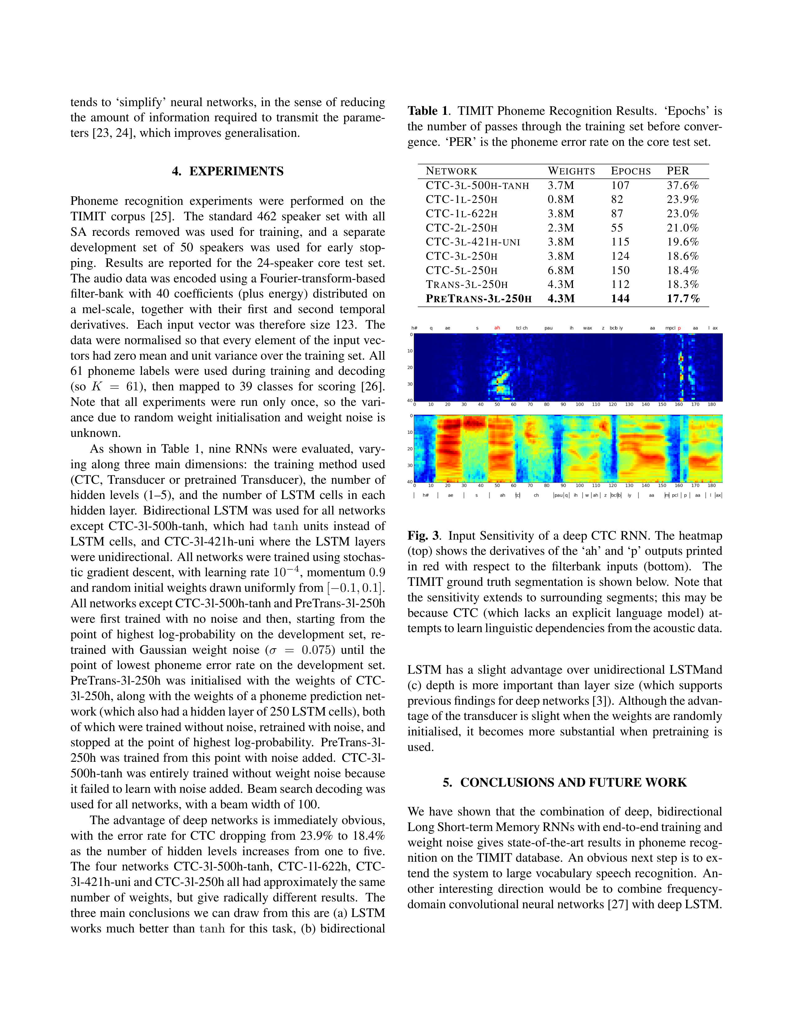
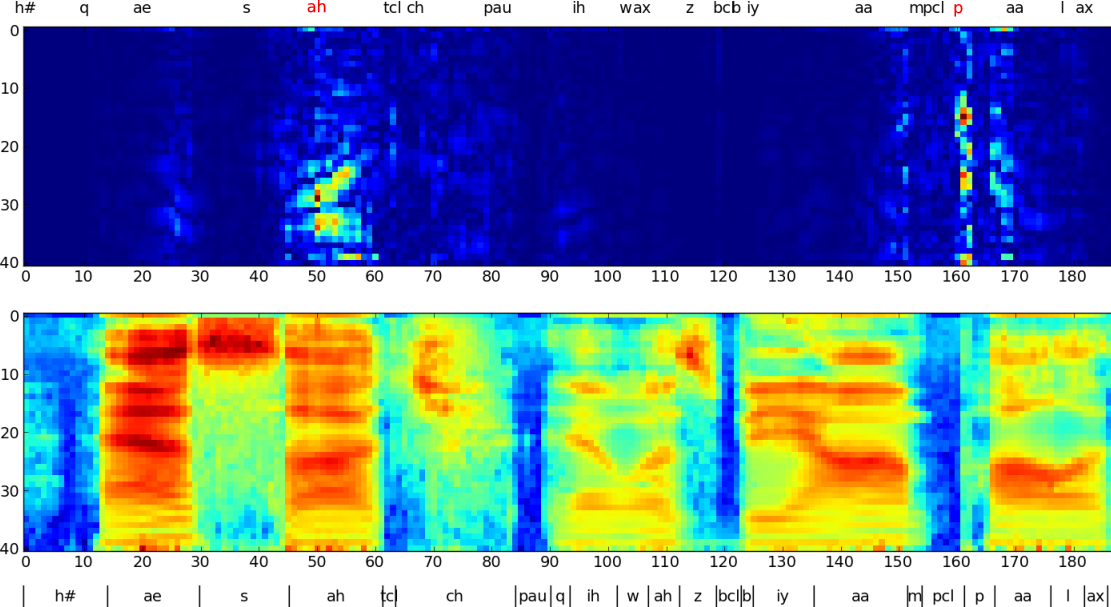
Fig.
3
.
Input
Sensitivity
of
a
deep
CTC
RNN.
The
heatmap
(top) shows the derivatives of the ‘ah’ and ‘p’ outputs printed
in
red
with
respect
to
the
filterbank
inputs
(bottom).
The
TIMIT ground truth segmentation is shown below.
Note that
the sensitivity extends to surrounding segments;
this may be
because
CTC
(which
lacks
an
explicit
language
model)
at-
tempts to learn linguistic dependencies from the acoustic data.
LSTM
has
a
slight
advantage
over
unidirectional
LSTMand
(c)
depth
is
more
important
than
layer
size
(which
supports
previous findings for deep networks [3]). Although the advan-
tage of the transducer is slight when the weights are randomly
initialised,
it
becomes
more
substantial
when
pretraining
is
used.
5.
CONCLUSIONS AND FUTURE WORK
We
have
shown
that
the
combination
of
deep,
bidirectional
Long Short-term Memory RNNs with end-to-end training and
weight noise gives state-of-the-art results in phoneme recog-
nition on the TIMIT database.
An obvious next step is to ex-
tend the system to large vocabulary speech recognition.
An-
other
interesting
direction
would
be
to
combine
frequency-
domain convolutional neural networks [27] with deep LSTM.
6.
REFERENCES
[1]
H.A.
Bourlard
and
N.
Morgan,
Connnectionist
Speech
Recognition:
A
Hybrid
Approach
,
Kluwer
Academic
Publishers, 1994.
[2]
Qifeng Zhu, Barry Chen, Nelson Morgan, and Andreas
Stolcke,
“Tandem
connectionist
feature
extraction
for
conversational
speech
recognition,”
in
International
Conference on Machine Learning for Multimodal Inter-
action
,
Berlin,
Heidelberg,
2005,
MLMI’04,
pp.
223–
231, Springer-Verlag.
[3]
A.
Mohamed,
G.E.
Dahl,
and
G.
Hinton,
“Acoustic
modeling
using
deep
belief
networks,”
Audio,
Speech,
and
Language
Processing,
IEEE
Transactions
on
,
vol.
20, no. 1, pp. 14 –22, jan. 2012.
[4]
G. Hinton, Li Deng, Dong Yu, G.E. Dahl, A. Mohamed,
N.
Jaitly,
A.
Senior,
V.
Vanhoucke,
P.
Nguyen,
T.N.
Sainath,
and
B.
Kingsbury,
“Deep
neural
networks
for
acoustic
modeling
in
speech
recognition,”
Signal
Pro-
cessing Magazine, IEEE
, vol. 29, no. 6, pp. 82 –97, nov.
2012.
[5]
A.
J.
Robinson,
“An
Application
of
Recurrent
Nets
to
Phone
Probability
Estimation,”
IEEE
Transactions
on
Neural Networks
, vol. 5, no. 2, pp. 298–305, 1994.
[6]
Oriol
Vinyals,
Suman
Ravuri,
and
Daniel
Povey,
“Re-
visiting
Recurrent
Neural
Networks
for
Robust
ASR,”
in
ICASSP
, 2012.
[7]
A. Maas,
Q. Le,
T. O’Neil,
O. Vinyals,
P. Nguyen,
and
A. Ng,
“Recurrent neural networks for noise reduction
in robust asr,”
in
INTERSPEECH
, 2012.
[8]
A. Graves, S. Fern´andez, F. Gomez, and J. Schmidhuber,
“Connectionist
Temporal
Classification:
Labelling
Un-
segmented
Sequence
Data
with
Recurrent
Neural
Net-
works,”
in
ICML
, Pittsburgh, USA, 2006.
[9]
A. Graves,
Supervised sequence labelling with recurrent
neural networks
, vol. 385,
Springer, 2012.
[10]
A. Graves,
“Sequence transduction with recurrent neu-
ral networks,”
in
ICML Representation Learning Work-
sop
, 2012.
[11]
S.
Hochreiter
and
J.
Schmidhuber,
“Long
Short-Term
Memory,”
Neural Computation
, vol. 9, no. 8, pp. 1735–
1780, 1997.
[12]
A.
Graves,
S.
Fern´andez,
M.
Liwicki,
H.
Bunke,
and
J.
Schmidhuber,
“Unconstrained
Online
Handwriting
Recognition with Recurrent Neural Networks,” in
NIPS
.
2008.
[13]
Alex Graves and Juergen Schmidhuber,
“Offline Hand-
writing
Recognition
with
Multidimensional
Recurrent
Neural Networks,”
in
NIPS
. 2009.
[14]
F. Gers, N. Schraudolph, and J. Schmidhuber, “Learning
Precise Timing with LSTM Recurrent Networks,”
Jour-
nal of Machine Learning Research
, vol. 3, pp. 115–143,
2002.
[15]
M.
Schuster
and
K.
K.
Paliwal,
“Bidirectional
Recur-
rent
Neural
Networks,”
IEEE
Transactions
on
Signal
Processing
, vol. 45, pp. 2673–2681, 1997.
[16]
A.
Graves
and
J.
Schmidhuber,
“Framewise
Phoneme
Classification with Bidirectional LSTM and Other Neu-
ral
Network
Architectures,”
Neural
Networks
,
vol.
18,
no. 5-6, pp. 602–610, June/July 2005.
[17]
David
E.
Rumelhart,
Geoffrey
E.
Hinton,
and
Ronald J. Williams,
Learning representations by back-
propagating errors
, pp. 696–699,
MIT Press, 1988.
[18]
Georey
Zweig
and
Patrick
Nguyen,
“SCARF:
A
seg-
mental
CRF
speech
recognition
system,”
Tech.
Rep.,
Microsoft Research, 2009.
[19]
Andrew W. Senior and Anthony J. Robinson, “Forward-
backward
retraining
of
recurrent
neural
networks,”
in
NIPS
, 1995, pp. 743–749.
[20]
Abdel rahman Mohamed,
Dong Yu,
and Li Deng,
“In-
vestigation of full-sequence training of deep belief net-
works for speech recognition,”
in
in Interspeech
, 2010.
[21]
M.
Lehr
and
I.
Shafran,
“Discriminatively
estimated
joint acoustic, duration, and language model for speech
recognition,”
in
ICASSP
, 2010, pp. 5542 –5545.
[22]
Kam-Chuen Jim, C.L. Giles, and B.G. Horne,
“An anal-
ysis of noise in recurrent neural networks:
convergence
and
generalization,”
Neural
Networks,
IEEE
Transac-
tions on
, vol. 7, no. 6, pp. 1424 –1438, nov 1996.
[23]
Geoffrey E. Hinton and Drew van Camp,
“Keeping the
neural
networks
simple
by
minimizing
the
description
length of the weights,”
in
COLT
, 1993, pp. 5–13.
[24]
Alex Graves,
“Practical variational inference for neural
networks,”
in
NIPS
, pp. 2348–2356. 2011.
[25]
DARPA-ISTO,
The
DARPA
TIMIT
Acoustic-Phonetic
Continuous
Speech
Corpus
(TIMIT)
,
speech
disc
cd1-
1.1 edition, 1990.
[26]
Kai fu Lee and Hsiao wuen Hon,
“Speaker-independent
phone recognition using hidden markov models,”
IEEE
Transactions on Acoustics, Speech, and Signal Process-
ing
, 1989.
[27]
O. Abdel-Hamid, A. Mohamed, Hui Jiang, and G. Penn,
“Applying
convolutional
neural
networks
concepts
to
hybrid
nn-hmm
model
for
speech
recognition,”
in
ICASSP
, march 2012, pp. 4277 –4280.