
On
the
Non-decoupling
of
Supervised
Fine-tuning
and
Reinforcement
Learning
in
Post-training
Xueyan
Niu
niuxueyan3@huawei.com
Theory
Laboratory
Central
Research
Institute,
2012
Laboratories
Huawei
Technologies
Co.,
Ltd.
Bo
Bai
baibo8@huawei.com
Wei
Han
harvey.hanwei@huawei.com
Weixi
Zhang
zhangweixi1@huawei.com
Abstract
Post-training
of
large
language
models
routinely
interleaves
supervised
fine-tuning
(SFT)
with
reinforcement
learning
(RL).
These
two
methods
have
different
objectives:
SFT
min-
imizes
the
cross-entropy
loss
between
model
outputs
and
expert
responses,
while
RL
max-
imizes
reward
signals
derived
from
human
preferences
or
rule-based
verifiers.
Modern
reasoning
models
have
widely
adopted
the
practice
of
alternating
SFT
and
RL
training.
However,
there
is
no
theoretical
account
of
whether
they
can
be
decoupled.
We
prove
that
decoupling
is
impossible
in
either
order:
(1)
SFT-then-RL
coupling:
RL
increases
SFT
loss under both distributional (KL-based) and landscape (PL-based) analyses;
and (2) RL-
then-SFT
coupling:
SFT
lowers
the
reward
achieved
by
RL
under
analogous
conditions.
Under
the
PL
condition,
we
further
derive
the
optimal
RL
duration
that
balances
reward
improvement
against
SFT
degradation,
identify
the
non-decoupling
threshold
governing
when
RL
can
improve
SFT,
and
bound
the
gradient
misalignment
via
spectral
concentra-
tion.
Experiments
on
Qwen3-0.6B
confirm
the
predicted
degradation,
verifying
that
SFT
and RL cannot be separated without loss of prior performance in the post-training pipeline.
1
Introduction
The
capacity
for
reasoning
and
general
tasks
has
been
greatly
improved
in
contemporary
Large
Language
Models
(LLMs)
thanks
to
post-training
techniques
such
as
Supervised
Fine-Tuning
(SFT)
and
Reinforcement
Learning
(RL).
Training
LLMs
typically
comprises
two
stages,
self-supervised
pretraining
and
post-training
,
as
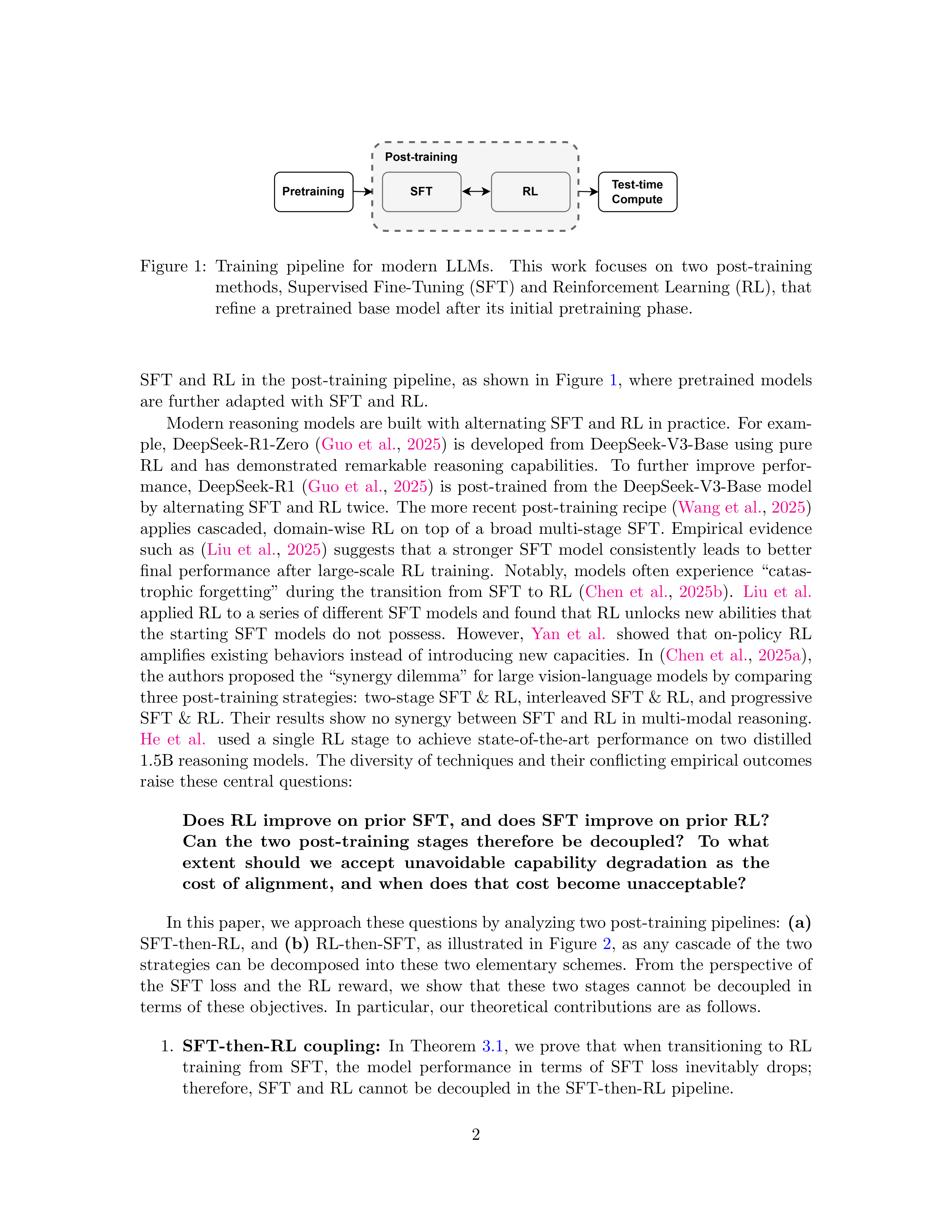
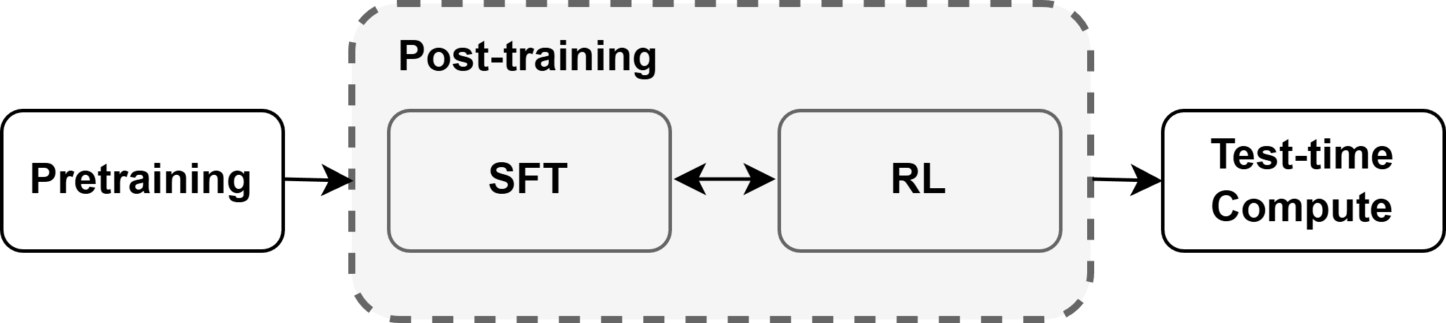
illustrated
in
Figure
1
.
Test-
time
strategies
can
also
be
applied
to
improve
the
performance
of
post-trained
models,
but
they
do
not
modify
the
parameters
of
the
post-trained
model.
During
the
pretraining
stage, the model acquires general language patterns, structure, grammar, factual knowledge,
and
reasoning
abilities
by
processing
vast
amounts
of
textual
data.
This
stage
of
LLM
training
demands
substantial
computational
resources.
In
addition,
it
involves
extensive
data
cleaning
to
ensure
that
the
model
learns
effectively
and
safely.
Post-training
often
involves
a
combination
of
SFT
and
RL.
SFT
is
a
process
that
teaches
the
model
how
to
respond
to
user
prompts
by
providing
task-specific
input-output
pairs,
while
the
RL
stage
encourages
certain
patterns
of
text
that
have
been
positively
reinforced
by
humans
or
rule-
based
verifiers.
SFT
has
been
shown
to
be
prone
to
memorization,
while
RL
is
related
to
generalization
(
Chu
et
al.
,
2025
;
Huan
et
al.
,
2025
).
In
this
work,
we
study
the
synergy
of
1
arXiv:2601.07389v2 [cs.LG] 6 May 2026
Figure
1:
Training
pipeline
for
modern
LLMs.
This
work
focuses
on
two
post-training
methods,
Supervised Fine-Tuning (SFT) and Reinforcement Learning (RL), that
refine
a
pretrained
base
model
after
its
initial
pretraining
phase.
SFT
and
RL
in
the
post-training
pipeline,
as
shown
in
Figure
1
,
where
pretrained
models
are
further
adapted
with
SFT
and
RL.
Modern reasoning models are built with alternating SFT and RL in practice.
For exam-
ple,
DeepSeek-R1-Zero
(
Guo
et
al.
,
2025
)
is
developed
from
DeepSeek-V3-Base
using
pure
RL
and
has
demonstrated
remarkable
reasoning
capabilities.
To
further
improve
perfor-
mance,
DeepSeek-R1
(
Guo
et
al.
,
2025
)
is
post-trained
from
the
DeepSeek-V3-Base
model
by alternating SFT and RL twice.
The more recent post-training recipe (
Wang et al.
,
2025
)
applies
cascaded,
domain-wise
RL
on
top
of
a
broad
multi-stage
SFT.
Empirical
evidence
such
as
(
Liu
et
al.
,
2025
)
suggests
that
a
stronger
SFT
model
consistently
leads
to
better
final
performance
after
large-scale
RL
training.
Notably,
models
often
experience
“catas-
trophic
forgetting”
during
the
transition
from
SFT
to
RL
(
Chen
et
al.
,
2025b
).
Liu
et
al.
applied RL to a series of different SFT models and found that RL unlocks new abilities that
the
starting
SFT
models
do
not
possess.
However,
Yan
et
al.
showed
that
on-policy
RL
amplifies
existing
behaviors
instead
of
introducing
new
capacities.
In
(
Chen
et
al.
,
2025a
),
the authors proposed the “synergy dilemma” for large vision-language models by comparing
three post-training strategies:
two-stage SFT & RL, interleaved SFT & RL, and progressive
SFT
&
RL.
Their
results
show
no
synergy
between
SFT
and
RL
in
multi-modal
reasoning.
He
et
al.
used
a
single
RL
stage
to
achieve
state-of-the-art
performance
on
two
distilled
1.5B reasoning models.
The diversity of techniques and their conflicting empirical outcomes
raise
these
central
questions:
Does
RL
improve
on
prior
SFT,
and
does
SFT
improve
on
prior
RL?
Can
the
two
post-training
stages
therefore
be
decoupled?
To
what
extent
should
we
accept
unavoidable
capability
degradation
as
the
cost
of
alignment,
and
when
does
that
cost
become
unacceptable?
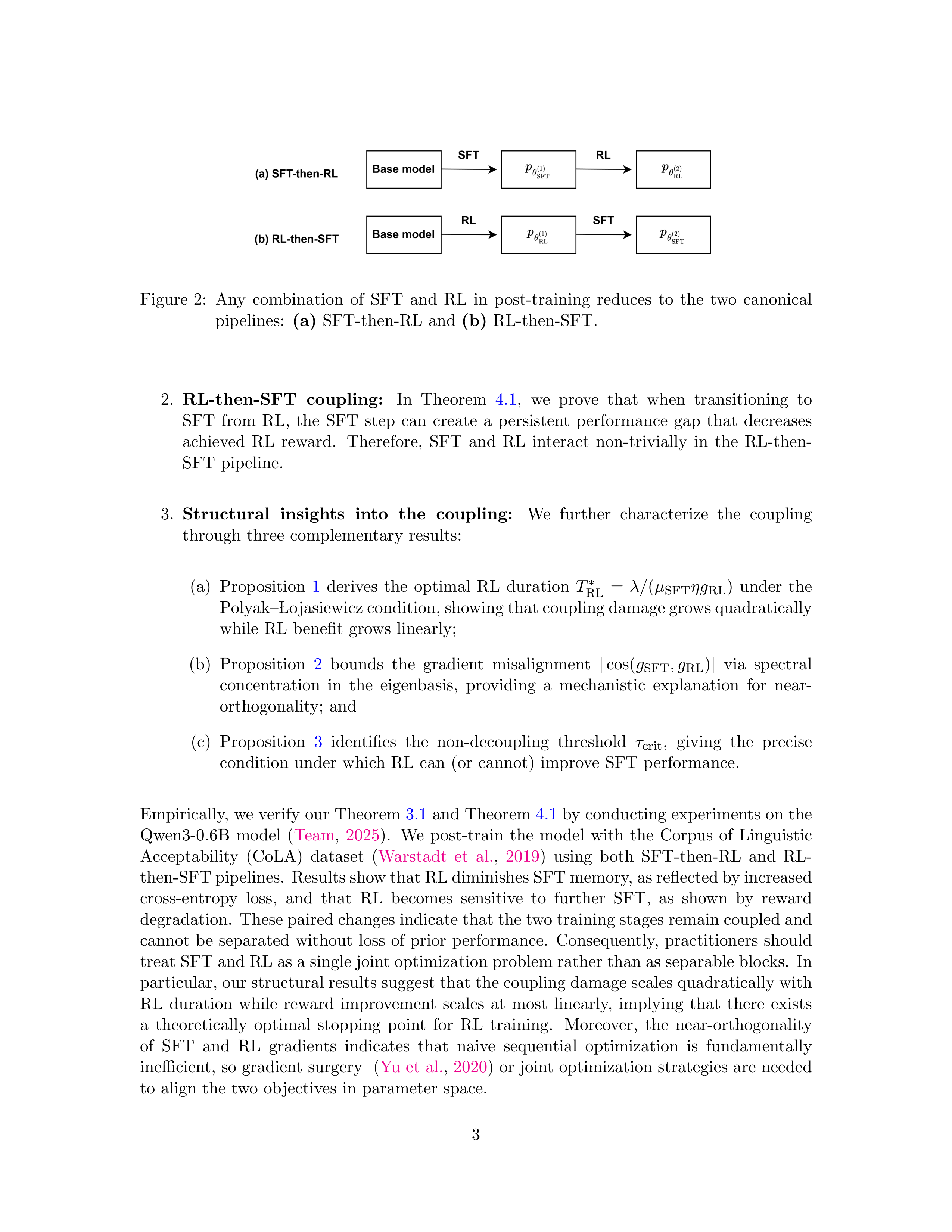
In this paper, we approach these questions by analyzing two post-training pipelines:
(a)
SFT-then-RL,
and
(b)
RL-then-SFT,
as
illustrated
in
Figure
2
,
as
any
cascade
of
the
two
strategies
can
be
decomposed
into
these
two
elementary
schemes.
From
the
perspective
of
the
SFT
loss
and
the
RL
reward,
we
show
that
these
two
stages
cannot
be
decoupled
in
terms
of
these
objectives.
In
particular,
our
theoretical
contributions
are
as
follows.
1.
SFT-then-RL
coupling:
In
Theorem
3.1
,
we
prove
that
when
transitioning
to
RL
training
from
SFT,
the
model
performance
in
terms
of
SFT
loss
inevitably
drops;
therefore,
SFT
and
RL
cannot
be
decoupled
in
the
SFT-then-RL
pipeline.
2
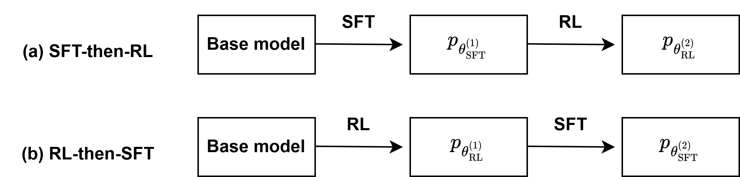
Figure
2:
Any
combination
of
SFT
and
RL
in
post-training
reduces
to
the
two
canonical
pipelines:
(a)
SFT-then-RL
and
(b)
RL-then-SFT.
2.
RL-then-SFT
coupling:
In
Theorem
4.1
,
we
prove
that
when
transitioning
to
SFT
from
RL,
the
SFT
step
can
create
a
persistent
performance
gap
that
decreases
achieved
RL
reward.
Therefore,
SFT
and
RL
interact
non-trivially
in
the
RL-then-
SFT
pipeline.
3.
Structural
insights
into
the
coupling:
We
further
characterize
the
coupling
through
three
complementary
results:
(a)
Proposition
1
derives
the
optimal
RL
duration
T
∗
RL
=
λ/
(
µ
SFT
η
¯
g
RL
)
under
the
Polyak–
Lojasiewicz condition, showing that coupling damage grows quadratically
while
RL
benefit
grows
linearly;
(b)
Proposition
2
bounds
the
gradient
misalignment
|
cos(
g
SFT
, g
RL
)
|
via
spectral
concentration
in
the
eigenbasis,
providing
a
mechanistic
explanation
for
near-
orthogonality;
and
(c)
Proposition
3
identifies
the
non-decoupling
threshold
τ
crit
,
giving
the
precise
condition
under
which
RL
can
(or
cannot)
improve
SFT
performance.
Empirically,
we verify our Theorem
3.1
and Theorem
4.1
by conducting experiments on the
Qwen3-0.6B
model
(
Team
,
2025
).
We
post-train
the
model
with
the
Corpus
of
Linguistic
Acceptability
(CoLA)
dataset
(
Warstadt
et
al.
,
2019
)
using
both
SFT-then-RL
and
RL-
then-SFT pipelines.
Results show that RL diminishes SFT memory, as reflected by increased
cross-entropy
loss,
and
that
RL
becomes
sensitive
to
further
SFT,
as
shown
by
reward
degradation.
These paired changes indicate that the two training stages remain coupled and
cannot
be
separated
without
loss
of
prior
performance.
Consequently,
practitioners
should
treat SFT and RL as a single joint optimization problem rather than as separable blocks.
In
particular, our structural results suggest that the coupling damage scales quadratically with
RL
duration
while
reward
improvement
scales
at
most
linearly,
implying
that
there
exists
a
theoretically
optimal
stopping
point
for
RL
training.
Moreover,
the
near-orthogonality
of
SFT
and
RL
gradients
indicates
that
naive
sequential
optimization
is
fundamentally
inefficient,
so
gradient
surgery
(
Yu
et
al.
,
2020
)
or
joint
optimization
strategies
are
needed
to
align
the
two
objectives
in
parameter
space.
3
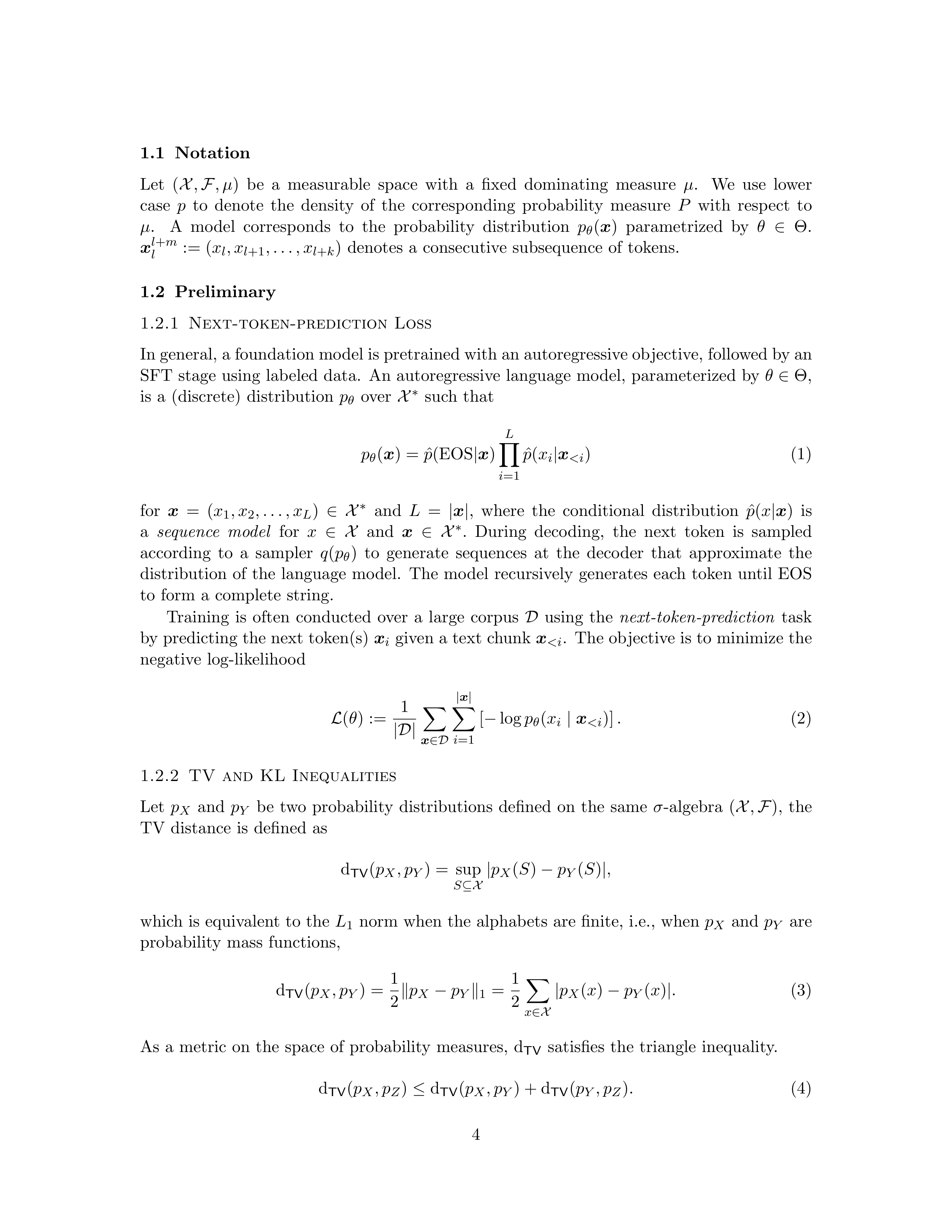
1.1
Notation
Let
(
X
,
F
, µ
)
be
a
measurable
space
with
a
fixed
dominating
measure
µ
.
We
use
lower
case
p
to
denote
the
density
of
the
corresponding
probability
measure
P
with
respect
to
µ
.
A
model
corresponds
to
the
probability
distribution
p
θ
(
x
)
parametrized
by
θ
∈
Θ
.
x
l
+
m
l
:= (
x
l
, x
l
+1
, . . . , x
l
+
k
)
denotes
a
consecutive
subsequence
of
tokens.
1.2
Preliminary
1.2.1
Next-token-prediction
Loss
In general, a foundation model is pretrained with an autoregressive objective, followed by an
SFT
stage
using
labeled
data.
An
autoregressive
language
model,
parameterized
by
θ
∈
Θ
,
is
a
(discrete)
distribution
p
θ
over
X
∗
such
that
p
θ
(
x
) =
ˆ
p
(EOS
|
x
)
L
Y
i
=1
ˆ
p
(
x
i
|
x
<i
)
(1)
for
x
=
(
x
1
, x
2
, . . . , x
L
)
∈X
∗
and
L
=
|
x
|
,
where
the
conditional
distribution
ˆ
p
(
x
|
x
)
is
a
sequence
model
for
x
∈X
and
x
∈X
∗
.
During
decoding,
the
next
token
is
sampled
according
to
a
sampler
q
(
p
θ
)
to
generate
sequences
at
the
decoder
that
approximate
the
distribution
of
the
language
model.
The
model
recursively
generates
each
token
until
EOS
to
form
a
complete
string.
Training
is
often
conducted
over
a
large
corpus
D
using
the
next-token-prediction
task
by predicting the next token(s)
x
i
given a text chunk
x
<i
.
The objective is to minimize the
negative
log-likelihood
L
(
θ
) :=
1
|D|
X
x
∈D
|
x
|
X
i
=1
[
−
log
p
θ
(
x
i
|
x
<i
)]
.
(2)
1.2.2
TV
and
KL
Inequalities
Let
p
X
and
p
Y
be
two
probability
distributions
defined
on
the
same
σ
-algebra
(
X
,
F
)
,
the
TV
distance
is
defined
as
d
TV
(
p
X
, p
Y
) =
sup
S
⊆X
|
p
X
(
S
)
−
p
Y
(
S
)
|
,
which
is
equivalent
to
the
L
1
norm
when
the
alphabets
are
finite,
i.e.,
when
p
X
and
p
Y
are
probability
mass
functions,
d
TV
(
p
X
, p
Y
) =
1
2
∥
p
X
−
p
Y
∥
1
=
1
2
X
x
∈X
|
p
X
(
x
)
−
p
Y
(
x
)
|
.
(3)
As
a
metric
on
the
space
of
probability
measures,
d
TV
satisfies
the
triangle
inequality.
d
TV
(
p
X
, p
Z
)
≤
d
TV
(
p
X
, p
Y
) + d
TV
(
p
Y
, p
Z
)
.
(4)
4
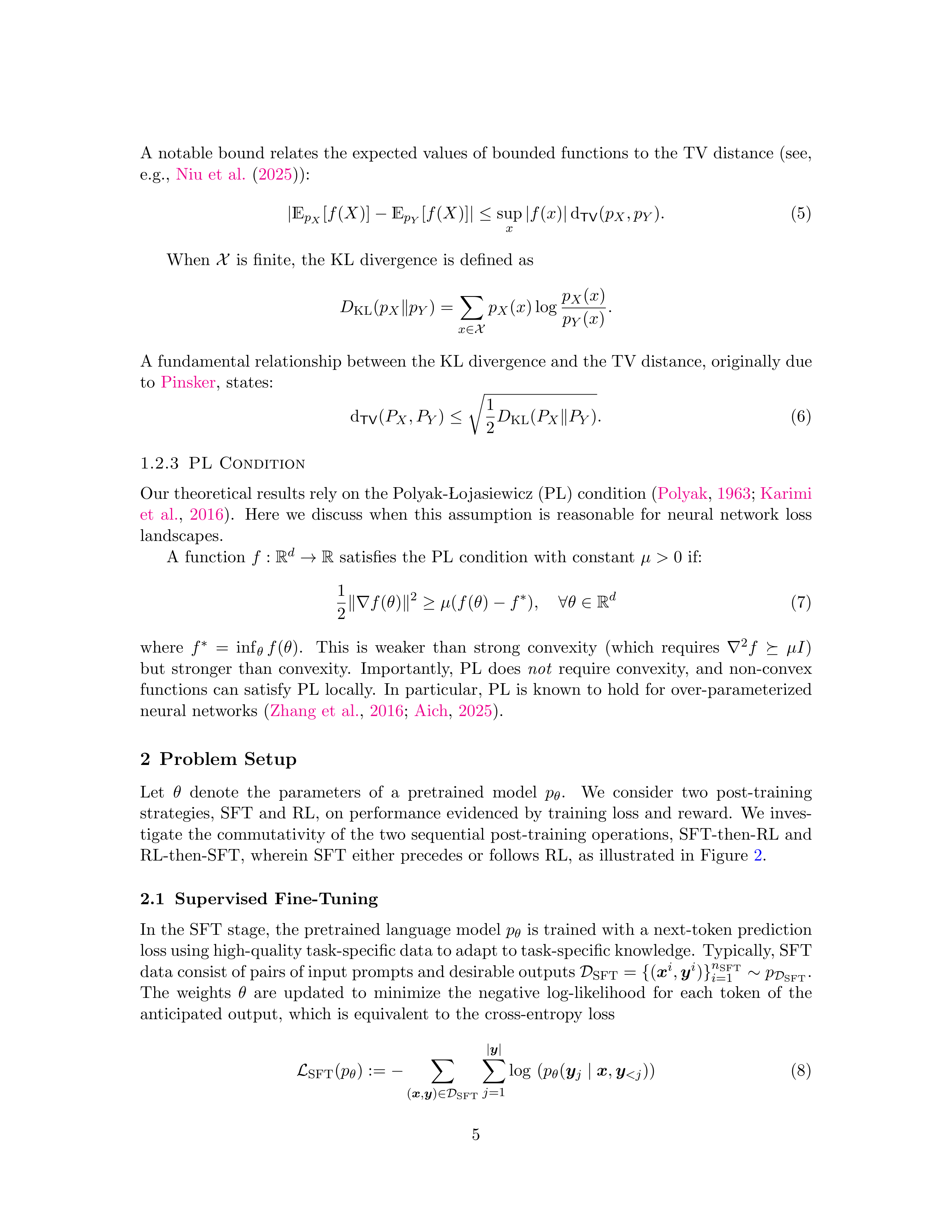
A
notable
bound
relates
the
expected
values
of
bounded
functions
to
the
TV
distance
(see,
e.g.,
Niu
et
al.
(
2025
)):
|
E
p
X
[
f
(
X
)]
−
E
p
Y
[
f
(
X
)]
| ≤
sup
x
|
f
(
x
)
|
d
TV
(
p
X
, p
Y
)
.
(5)
When
X
is
finite,
the
KL
divergence
is
defined
as
D
KL
(
p
X
∥
p
Y
) =
X
x
∈X
p
X
(
x
) log
p
X
(
x
)
p
Y
(
x
)
.
A fundamental relationship between the KL divergence and the TV distance, originally due
to
Pinsker
,
states:
d
TV
(
P
X
, P
Y
)
≤
r
1
2
D
KL
(
P
X
∥
P
Y
)
.
(6)
1.2.3
PL
Condition
Our theoretical results rely on the Polyak-
Lojasiewicz (PL) condition (
Polyak
,
1963
;
Karimi
et
al.
,
2016
).
Here
we
discuss
when
this
assumption
is
reasonable
for
neural
network
loss
landscapes.
A
function
f
:
R
d
→
R
satisfies
the
PL
condition
with
constant
µ >
0
if:
1
2
∥∇
f
(
θ
)
∥
2
≥
µ
(
f
(
θ
)
−
f
∗
)
,
∀
θ
∈
R
d
(7)
where
f
∗
=
inf
θ
f
(
θ
).
This
is
weaker
than
strong
convexity
(which
requires
∇
2
f
⪰
µI
)
but
stronger
than
convexity.
Importantly,
PL
does
not
require
convexity,
and
non-convex
functions
can
satisfy
PL
locally.
In
particular,
PL
is
known
to
hold
for
over-parameterized
neural
networks
(
Zhang
et
al.
,
2016
;
Aich
,
2025
).
2
Problem
Setup
Let
θ
denote
the
parameters
of
a
pretrained
model
p
θ
.
We
consider
two
post-training
strategies,
SFT
and
RL,
on
performance
evidenced
by
training
loss
and
reward.
We
inves-
tigate
the
commutativity
of
the
two
sequential
post-training
operations,
SFT-then-RL
and
RL-then-SFT,
wherein
SFT
either
precedes
or
follows
RL,
as
illustrated
in
Figure
2
.
2.1
Supervised
Fine-Tuning
In
the
SFT
stage,
the
pretrained
language
model
p
θ
is
trained
with
a
next-token
prediction
loss using high-quality task-specific data to adapt to task-specific knowledge.
Typically, SFT
data consist of pairs of input prompts and desirable outputs
D
SFT
=
{
(
x
i
,
y
i
)
}
n
SFT
i
=1
∼
p
D
SFT
.
The
weights
θ
are
updated
to
minimize
the
negative
log-likelihood
for
each
token
of
the
anticipated
output,
which
is
equivalent
to
the
cross-entropy
loss
L
SFT
(
p
θ
) :=
−
X
(
x
,
y
)
∈D
SFT
|
y
|
X
j
=1
log
(
p
θ
(
y
j
|
x
,
y
<j
))
(8)
5
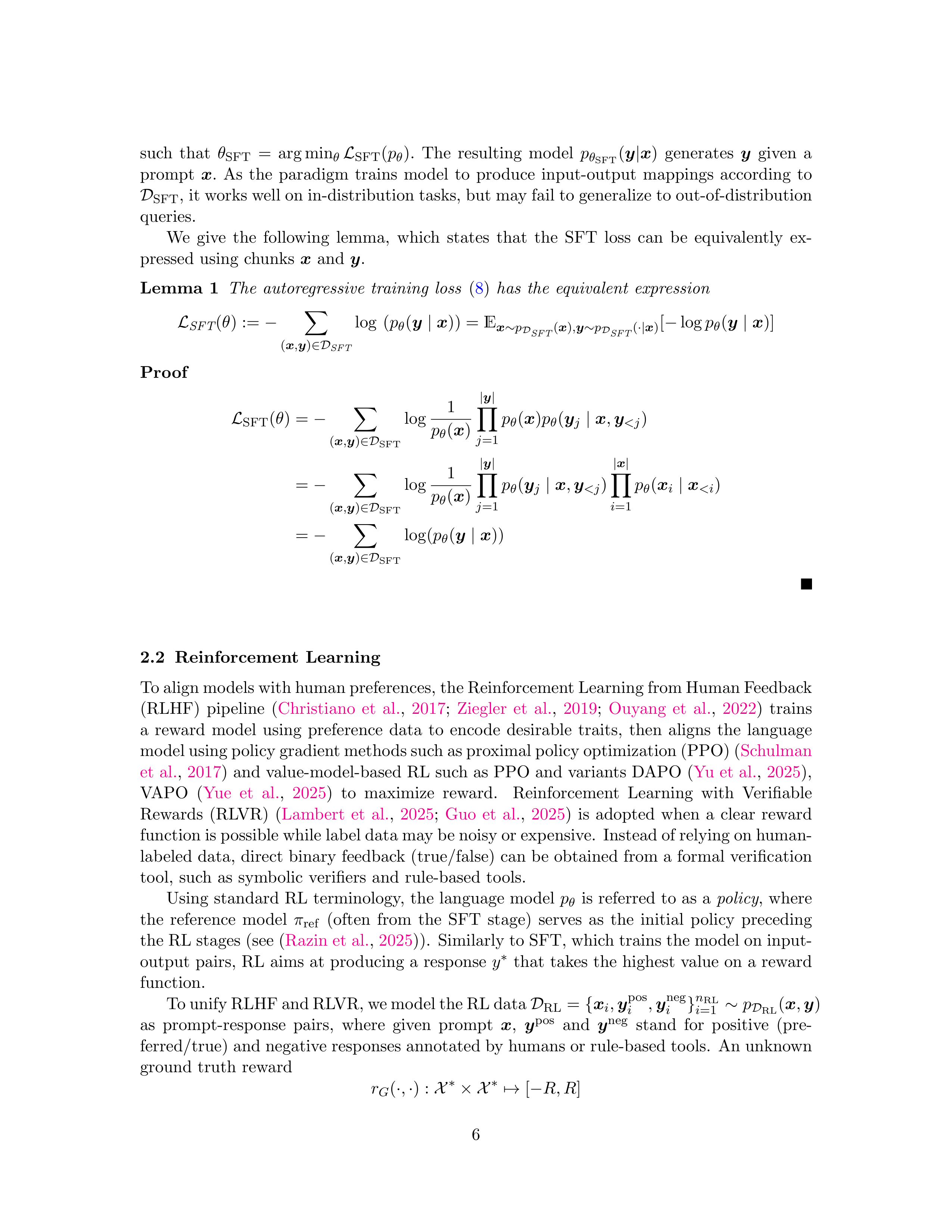
such
that
θ
SFT
=
arg min
θ
L
SFT
(
p
θ
)
.
The
resulting
model
p
θ
SFT
(
y
|
x
)
generates
y
given
a
prompt
x
.
As
the
paradigm
trains
model
to
produce
input-output
mappings
according
to
D
SFT
, it works well on in-distribution tasks, but may fail to generalize to out-of-distribution
queries.
We
give
the
following
lemma,
which
states
that
the
SFT
loss
can
be
equivalently
ex-
pressed
using
chunks
x
and
y
.
Lemma
1
The
autoregressive
training
loss
(
8
)
has
the
equivalent
expression
L
SFT
(
θ
) :=
−
X
(
x
,
y
)
∈D
SFT
log
(
p
θ
(
y
|
x
)) =
E
x
∼
p
D
SFT
(
x
)
,
y
∼
p
D
SFT
(
·|
x
)
[
−
log
p
θ
(
y
|
x
)]
Proof
L
SFT
(
θ
) =
−
X
(
x
,
y
)
∈D
SFT
log
1
p
θ
(
x
)
|
y
|
Y
j
=1
p
θ
(
x
)
p
θ
(
y
j
|
x
,
y
<j
)
=
−
X
(
x
,
y
)
∈D
SFT
log
1
p
θ
(
x
)
|
y
|
Y
j
=1
p
θ
(
y
j
|
x
,
y
<j
)
|
x
|
Y
i
=1
p
θ
(
x
i
|
x
<i
)
=
−
X
(
x
,
y
)
∈D
SFT
log(
p
θ
(
y
|
x
))
2.2
Reinforcement
Learning
To align models with human preferences, the Reinforcement Learning from Human Feedback
(RLHF)
pipeline
(
Christiano
et
al.
,
2017
;
Ziegler
et
al.
,
2019
;
Ouyang
et
al.
,
2022
)
trains
a
reward
model
using
preference
data
to
encode
desirable
traits,
then
aligns
the
language
model using policy gradient methods such as proximal policy optimization (PPO) (
Schulman
et
al.
,
2017
)
and
value-model-based
RL
such
as
PPO
and
variants
DAPO
(
Yu
et
al.
,
2025
),
VAPO
(
Yue
et
al.
,
2025
)
to
maximize
reward.
Reinforcement
Learning
with
Verifiable
Rewards
(RLVR)
(
Lambert
et
al.
,
2025
;
Guo
et
al.
,
2025
)
is
adopted
when
a
clear
reward
function is possible while label data may be noisy or expensive.
Instead of relying on human-
labeled
data,
direct
binary
feedback
(true/false)
can
be
obtained
from
a
formal
verification
tool,
such
as
symbolic
verifiers
and
rule-based
tools.
Using
standard
RL
terminology,
the
language
model
p
θ
is
referred
to
as
a
policy
,
where
the
reference
model
π
ref
(often
from
the
SFT
stage)
serves
as
the
initial
policy
preceding
the RL stages (see (
Razin et al.
,
2025
)).
Similarly to SFT, which trains the model on input-
output
pairs,
RL
aims
at
producing
a
response
y
∗
that
takes
the
highest
value
on
a
reward
function.
To unify RLHF and RLVR, we model the RL data
D
RL
=
{
x
i
,
y
pos
i
,
y
neg
i
}
n
RL
i
=1
∼
p
D
RL
(
x
,
y
)
as
prompt-response
pairs,
where
given
prompt
x
,
y
pos
and
y
neg
stand
for
positive
(pre-
ferred/true) and negative responses annotated by humans or rule-based tools.
An unknown
ground
truth
reward
r
G
(
·
,
·
) :
X
∗
× X
∗
7→
[
−
R, R
]
6
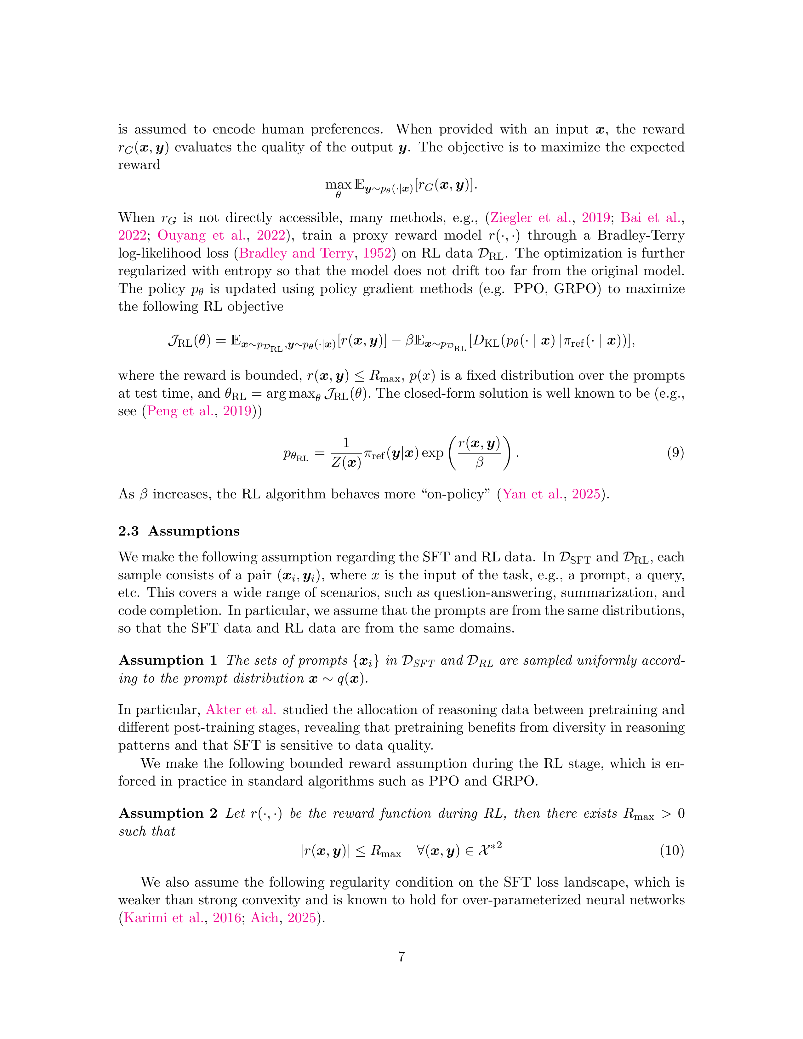
is
assumed
to
encode
human
preferences.
When
provided
with
an
input
x
,
the
reward
r
G
(
x
,
y
)
evaluates
the
quality
of
the
output
y
.
The
objective
is
to
maximize
the
expected
reward
max
θ
E
y
∼
p
θ
(
·|
x
)
[
r
G
(
x
,
y
)]
.
When
r
G
is
not
directly
accessible,
many
methods,
e.g.,
(
Ziegler
et
al.
,
2019
;
Bai
et
al.
,
2022
;
Ouyang
et
al.
,
2022
),
train
a
proxy
reward
model
r
(
·
,
·
)
through
a
Bradley-Terry
log-likelihood
loss
(
Bradley
and
Terry
,
1952
)
on
RL
data
D
RL
.
The
optimization
is
further
regularized
with
entropy
so
that
the
model
does
not
drift
too
far
from
the
original
model.
The
policy
p
θ
is
updated
using
policy
gradient
methods
(e.g.
PPO,
GRPO)
to
maximize
the
following
RL
objective
J
RL
(
θ
) =
E
x
∼
p
D
RL
,
y
∼
p
θ
(
·|
x
)
[
r
(
x
,
y
)]
−
β
E
x
∼
p
D
RL
[
D
KL
(
p
θ
(
· |
x
)
∥
π
ref
(
· |
x
))]
,
where
the
reward
is
bounded,
r
(
x
,
y
)
≤
R
max
,
p
(
x
)
is
a
fixed
distribution
over
the
prompts
at test time, and
θ
RL
= arg max
θ
J
RL
(
θ
)
.
The closed-form solution is well known to be (e.g.,
see
(
Peng
et
al.
,
2019
))
p
θ
RL
=
1
Z
(
x
)
π
ref
(
y
|
x
) exp
r
(
x
,
y
)
β
.
(9)
As
β
increases,
the
RL
algorithm
behaves
more
“on-policy”
(
Yan
et
al.
,
2025
).
2.3
Assumptions
We make the following assumption regarding the SFT and RL data.
In
D
SFT
and
D
RL
,
each
sample
consists
of
a
pair
(
x
i
,
y
i
)
,
where
x
is
the
input
of
the
task,
e.g.,
a
prompt,
a
query,
etc.
This
covers
a
wide
range
of
scenarios,
such
as
question-answering,
summarization,
and
code completion.
In particular, we assume that the prompts are from the same distributions,
so
that
the
SFT
data
and
RL
data
are
from
the
same
domains.
Assumption
1
The
sets
of
prompts
{
x
i
}
in
D
SFT
and
D
RL
are
sampled
uniformly
accord-
ing
to
the
prompt
distribution
x
∼
q
(
x
)
.
In
particular,
Akter
et
al.
studied
the
allocation
of
reasoning
data
between
pretraining
and
different post-training stages, revealing that pretraining benefits from diversity in reasoning
patterns
and
that
SFT
is
sensitive
to
data
quality.
We
make
the
following
bounded
reward
assumption
during
the
RL
stage,
which
is
en-
forced
in
practice
in
standard
algorithms
such
as
PPO
and
GRPO.
Assumption
2
Let
r
(
·
,
·
)
be
the
reward
function
during
RL,
then
there
exists
R
max
>
0
such
that
|
r
(
x
,
y
)
| ≤
R
max
∀
(
x
,
y
)
∈X
∗
2
(10)
We
also
assume
the
following
regularity
condition
on
the
SFT
loss
landscape,
which
is
weaker
than
strong
convexity
and
is
known
to
hold
for
over-parameterized
neural
networks
(
Karimi
et
al.
,
2016
;
Aich
,
2025
).
7
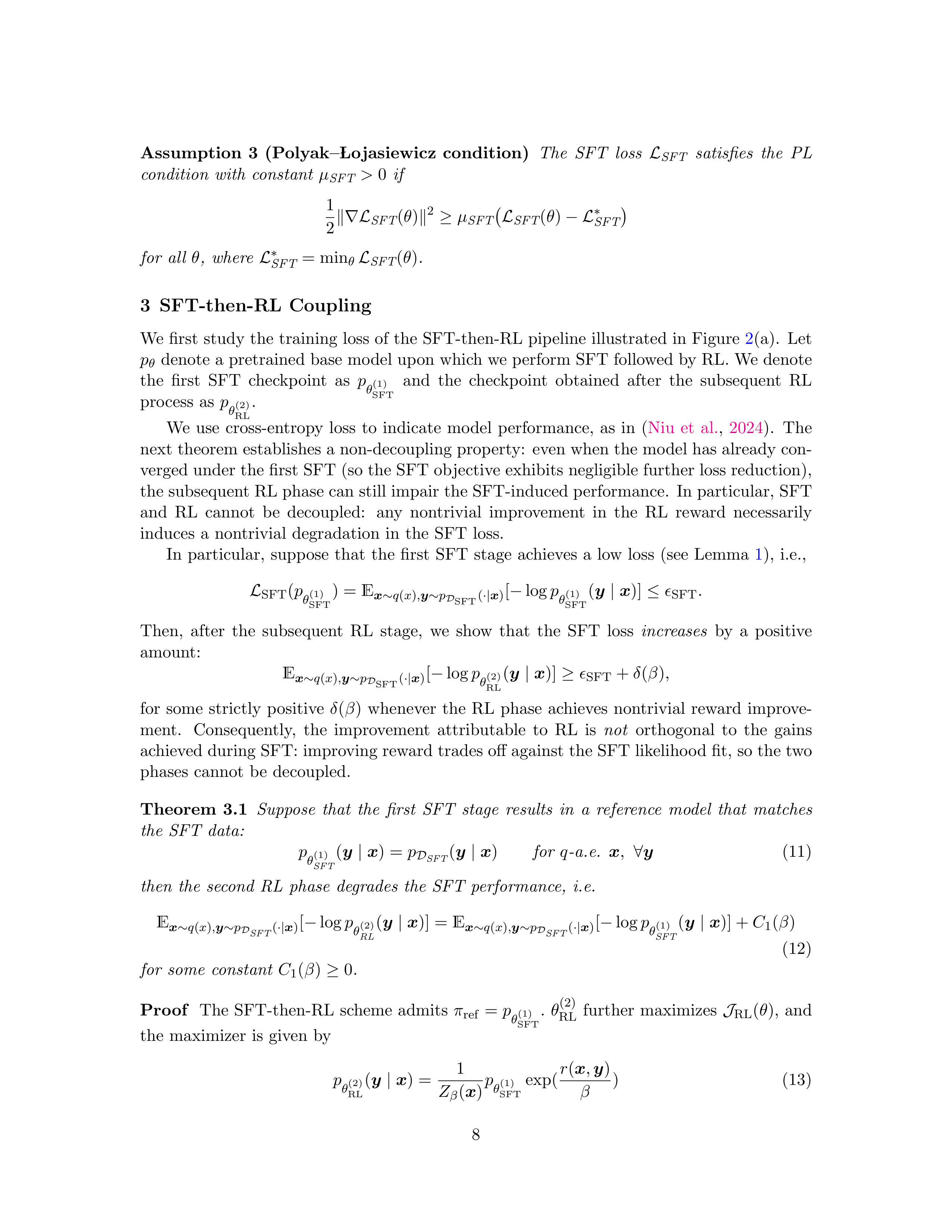
Assumption
3
(Polyak–
Lojasiewicz
condition)
The
SFT
loss
L
SFT
satisfies
the
PL
condition
with
constant
µ
SFT
>
0
if
1
2
∥∇L
SFT
(
θ
)
∥
2
≥
µ
SFT
L
SFT
(
θ
)
−L
∗
SFT
for
all
θ
,
where
L
∗
SFT
= min
θ
L
SFT
(
θ
)
.
3
SFT-then-RL
Coupling
We
first
study
the
training
loss
of
the
SFT-then-RL
pipeline
illustrated
in
Figure
2
(a).
Let
p
θ
denote
a
pretrained base
model
upon
which
we
perform
SFT
followed by RL.
We
denote
the
first
SFT
checkpoint
as
p
θ
(1)
SFT
and
the
checkpoint
obtained
after
the
subsequent
RL
process
as
p
θ
(2)
RL
.
We
use
cross-entropy
loss
to
indicate
model
performance,
as
in
(
Niu
et
al.
,
2024
).
The
next theorem establishes a non-decoupling property:
even when the model has already con-
verged under the first SFT (so the SFT objective exhibits negligible further loss reduction),
the subsequent RL phase can still impair the SFT-induced performance.
In particular, SFT
and
RL
cannot
be
decoupled:
any
nontrivial
improvement
in
the
RL
reward
necessarily
induces
a
nontrivial
degradation
in
the
SFT
loss.
In
particular,
suppose
that
the
first
SFT
stage
achieves
a
low
loss
(see
Lemma
1
),
i.e.,
L
SFT
(
p
θ
(1)
SFT
) =
E
x
∼
q
(
x
)
,
y
∼
p
D
SFT
(
·|
x
)
[
−
log
p
θ
(1)
SFT
(
y
|
x
)]
≤
ϵ
SFT
.
Then,
after
the
subsequent
RL
stage,
we
show
that
the
SFT
loss
increases
by
a
positive
amount:
E
x
∼
q
(
x
)
,
y
∼
p
D
SFT
(
·|
x
)
[
−
log
p
θ
(2)
RL
(
y
|
x
)]
≥
ϵ
SFT
+
δ
(
β
)
,
for
some
strictly
positive
δ
(
β
)
whenever
the
RL
phase
achieves
nontrivial
reward
improve-
ment.
Consequently,
the
improvement
attributable
to
RL
is
not
orthogonal
to
the
gains
achieved during SFT: improving reward trades off against the SFT likelihood fit, so the two
phases
cannot
be
decoupled.
Theorem
3.1
Suppose
that
the
first
SFT
stage
results
in
a
reference
model
that
matches
the
SFT
data:
p
θ
(1)
SFT
(
y
|
x
) =
p
D
SFT
(
y
|
x
)
for
q
-a.e.
x
,
∀
y
(11)
then
the
second
RL
phase
degrades
the
SFT
performance,
i.e.
E
x
∼
q
(
x
)
,
y
∼
p
D
SFT
(
·|
x
)
[
−
log
p
θ
(2)
RL
(
y
|
x
)] =
E
x
∼
q
(
x
)
,
y
∼
p
D
SFT
(
·|
x
)
[
−
log
p
θ
(1)
SFT
(
y
|
x
)] +
C
1
(
β
)
(12)
for
some
constant
C
1
(
β
)
≥
0
.
Proof
The
SFT-then-RL
scheme
admits
π
ref
=
p
θ
(1)
SFT
.
θ
(2)
RL
further
maximizes
J
RL
(
θ
),
and
the
maximizer
is
given
by
p
θ
(2)
RL
(
y
|
x
) =
1
Z
β
(
x
)
p
θ
(1)
SFT
exp(
r
(
x
,
y
)
β
)
(13)
8
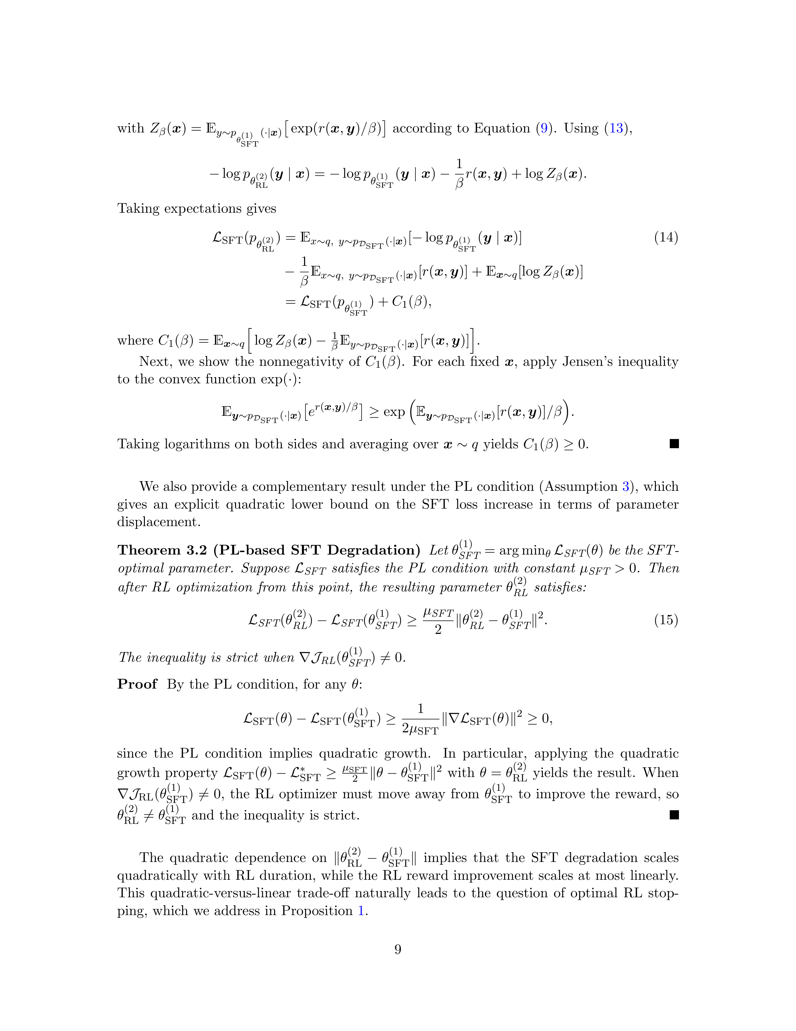
with
Z
β
(
x
) =
E
y
∼
p
θ
(1)
SFT
(
·|
x
)
exp(
r
(
x
,
y
)
/β
)
according
to
Equation
(
9
).
Using
(
13
),
−
log
p
θ
(2)
RL
(
y
|
x
) =
−
log
p
θ
(1)
SFT
(
y
|
x
)
−
1
β
r
(
x
,
y
) + log
Z
β
(
x
)
.
Taking
expectations
gives
L
SFT
(
p
θ
(2)
RL
) =
E
x
∼
q,
y
∼
p
D
SFT
(
·|
x
)
[
−
log
p
θ
(1)
SFT
(
y
|
x
)]
(14)
−
1
β
E
x
∼
q,
y
∼
p
D
SFT
(
·|
x
)
[
r
(
x
,
y
)] +
E
x
∼
q
[log
Z
β
(
x
)]
=
L
SFT
(
p
θ
(1)
SFT
) +
C
1
(
β
)
,
where
C
1
(
β
) =
E
x
∼
q
h
log
Z
β
(
x
)
−
1
β
E
y
∼
p
D
SFT
(
·|
x
)
[
r
(
x
,
y
)]
i
.
Next,
we
show
the
nonnegativity
of
C
1
(
β
).
For
each
fixed
x
,
apply
Jensen’s
inequality
to
the
convex
function
exp(
·
):
E
y
∼
p
D
SFT
(
·|
x
)
e
r
(
x
,
y
)
/β
≥
exp
E
y
∼
p
D
SFT
(
·|
x
)
[
r
(
x
,
y
)]
/β
.
Taking
logarithms
on
both
sides
and
averaging
over
x
∼
q
yields
C
1
(
β
)
≥
0.
We also provide
a complementary result under
the
PL condition (Assumption
3
),
which
gives
an
explicit
quadratic
lower
bound
on
the
SFT
loss
increase
in
terms
of
parameter
displacement.
Theorem
3.2
(PL-based
SFT
Degradation)
Let
θ
(1)
SFT
= arg min
θ
L
SFT
(
θ
)
be the SFT-
optimal
parameter.
Suppose
L
SFT
satisfies
the
PL
condition
with
constant
µ
SFT
>
0
.
Then
after
RL
optimization
from
this
point,
the
resulting
parameter
θ
(2)
RL
satisfies:
L
SFT
(
θ
(2)
RL
)
−L
SFT
(
θ
(1)
SFT
)
≥
µ
SFT
2
∥
θ
(2)
RL
−
θ
(1)
SFT
∥
2
.
(15)
The
inequality
is
strict
when
∇J
RL
(
θ
(1)
SFT
)
̸
= 0
.
Proof
By
the
PL
condition,
for
any
θ
:
L
SFT
(
θ
)
−L
SFT
(
θ
(1)
SFT
)
≥
1
2
µ
SFT
∥∇L
SFT
(
θ
)
∥
2
≥
0
,
since
the
PL
condition
implies
quadratic
growth.
In
particular,
applying
the
quadratic
growth
property
L
SFT
(
θ
)
−L
∗
SFT
≥
µ
SFT
2
∥
θ
−
θ
(1)
SFT
∥
2
with
θ
=
θ
(2)
RL
yields
the
result.
When
∇J
RL
(
θ
(1)
SFT
)
̸
=
0,
the
RL
optimizer
must
move
away
from
θ
(1)
SFT
to
improve
the
reward,
so
θ
(2)
RL
̸
=
θ
(1)
SFT
and
the
inequality
is
strict.
The
quadratic
dependence
on
∥
θ
(2)
RL
−
θ
(1)
SFT
∥
implies
that
the
SFT
degradation
scales
quadratically
with
RL
duration,
while
the
RL
reward
improvement
scales
at
most
linearly.
This
quadratic-versus-linear
trade-off
naturally
leads
to
the
question
of
optimal
RL
stop-
ping,
which
we
address
in
Proposition
1
.
9
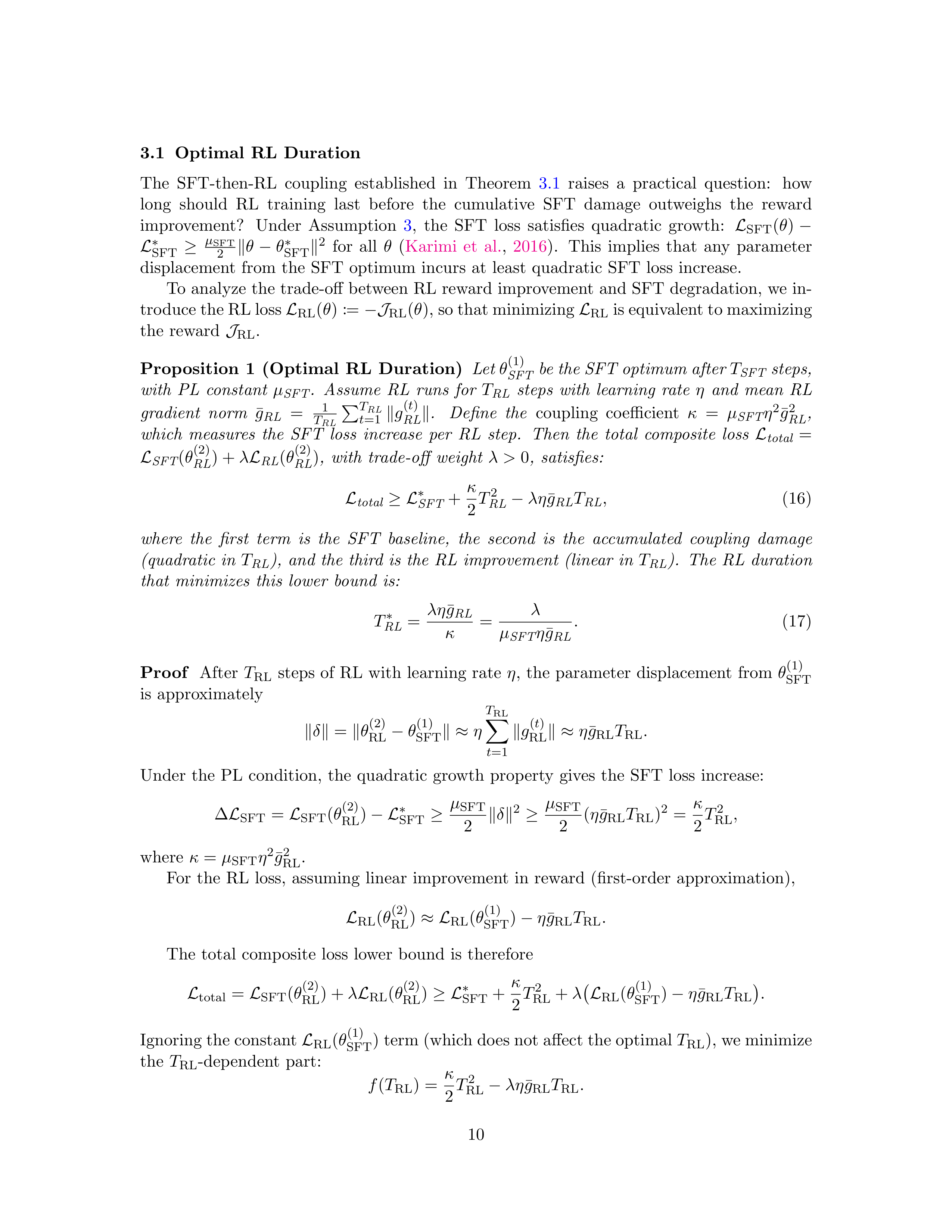
3.1
Optimal
RL
Duration
The
SFT-then-RL
coupling
established
in
Theorem
3.1
raises
a
practical
question:
how
long
should
RL
training
last
before
the
cumulative
SFT
damage
outweighs
the
reward
improvement?
Under
Assumption
3
,
the
SFT
loss
satisfies
quadratic
growth:
L
SFT
(
θ
)
−
L
∗
SFT
≥
µ
SFT
2
∥
θ
−
θ
∗
SFT
∥
2
for
all
θ
(
Karimi
et
al.
,
2016
).
This
implies
that
any
parameter
displacement
from
the
SFT
optimum
incurs
at
least
quadratic
SFT
loss
increase.
To
analyze
the
trade-off
between
RL
reward
improvement
and
SFT
degradation,
we
in-
troduce the RL loss
L
RL
(
θ
) :=
−J
RL
(
θ
), so that minimizing
L
RL
is equivalent to maximizing
the
reward
J
RL
.
Proposition
1
(Optimal
RL
Duration)
Let
θ
(1)
SFT
be the SFT optimum after
T
SFT
steps,
with
PL
constant
µ
SFT
.
Assume
RL
runs
for
T
RL
steps
with
learning
rate
η
and
mean
RL
gradient
norm
¯
g
RL
=
1
T
RL
P
T
RL
t
=1
∥
g
(
t
)
RL
∥
.
Define
the
coupling
coefficient
κ
=
µ
SFT
η
2
¯
g
2
RL
,
which
measures
the
SFT
loss
increase
per
RL
step.
Then
the
total
composite
loss
L
total
=
L
SFT
(
θ
(2)
RL
) +
λ
L
RL
(
θ
(2)
RL
)
,
with
trade-off
weight
λ >
0
,
satisfies:
L
total
≥L
∗
SFT
+
κ
2
T
2
RL
−
λη
¯
g
RL
T
RL
,
(16)
where
the
first
term
is
the
SFT
baseline,
the
second
is
the
accumulated
coupling
damage
(quadratic
in
T
RL
),
and
the
third
is
the
RL
improvement
(linear
in
T
RL
).
The
RL
duration
that
minimizes
this
lower
bound
is:
T
∗
RL
=
λη
¯
g
RL
κ
=
λ
µ
SFT
η
¯
g
RL
.
(17)
Proof
After
T
RL
steps
of
RL
with
learning
rate
η
,
the
parameter
displacement
from
θ
(1)
SFT
is
approximately
∥
δ
∥
=
∥
θ
(2)
RL
−
θ
(1)
SFT
∥≈
η
T
RL
X
t
=1
∥
g
(
t
)
RL
∥≈
η
¯
g
RL
T
RL
.
Under
the
PL
condition,
the
quadratic
growth
property
gives
the
SFT
loss
increase:
∆
L
SFT
=
L
SFT
(
θ
(2)
RL
)
−L
∗
SFT
≥
µ
SFT
2
∥
δ
∥
2
≥
µ
SFT
2
(
η
¯
g
RL
T
RL
)
2
=
κ
2
T
2
RL
,
where
κ
=
µ
SFT
η
2
¯
g
2
RL
.
For
the
RL
loss,
assuming
linear
improvement
in
reward
(first-order
approximation),
L
RL
(
θ
(2)
RL
)
≈L
RL
(
θ
(1)
SFT
)
−
η
¯
g
RL
T
RL
.
The
total
composite
loss
lower
bound
is
therefore
L
total
=
L
SFT
(
θ
(2)
RL
) +
λ
L
RL
(
θ
(2)
RL
)
≥L
∗
SFT
+
κ
2
T
2
RL
+
λ
L
RL
(
θ
(1)
SFT
)
−
η
¯
g
RL
T
RL
.
Ignoring the constant
L
RL
(
θ
(1)
SFT
) term (which does not affect the optimal
T
RL
), we minimize
the
T
RL
-dependent
part:
f
(
T
RL
) =
κ
2
T
2
RL
−
λη
¯
g
RL
T
RL
.
10
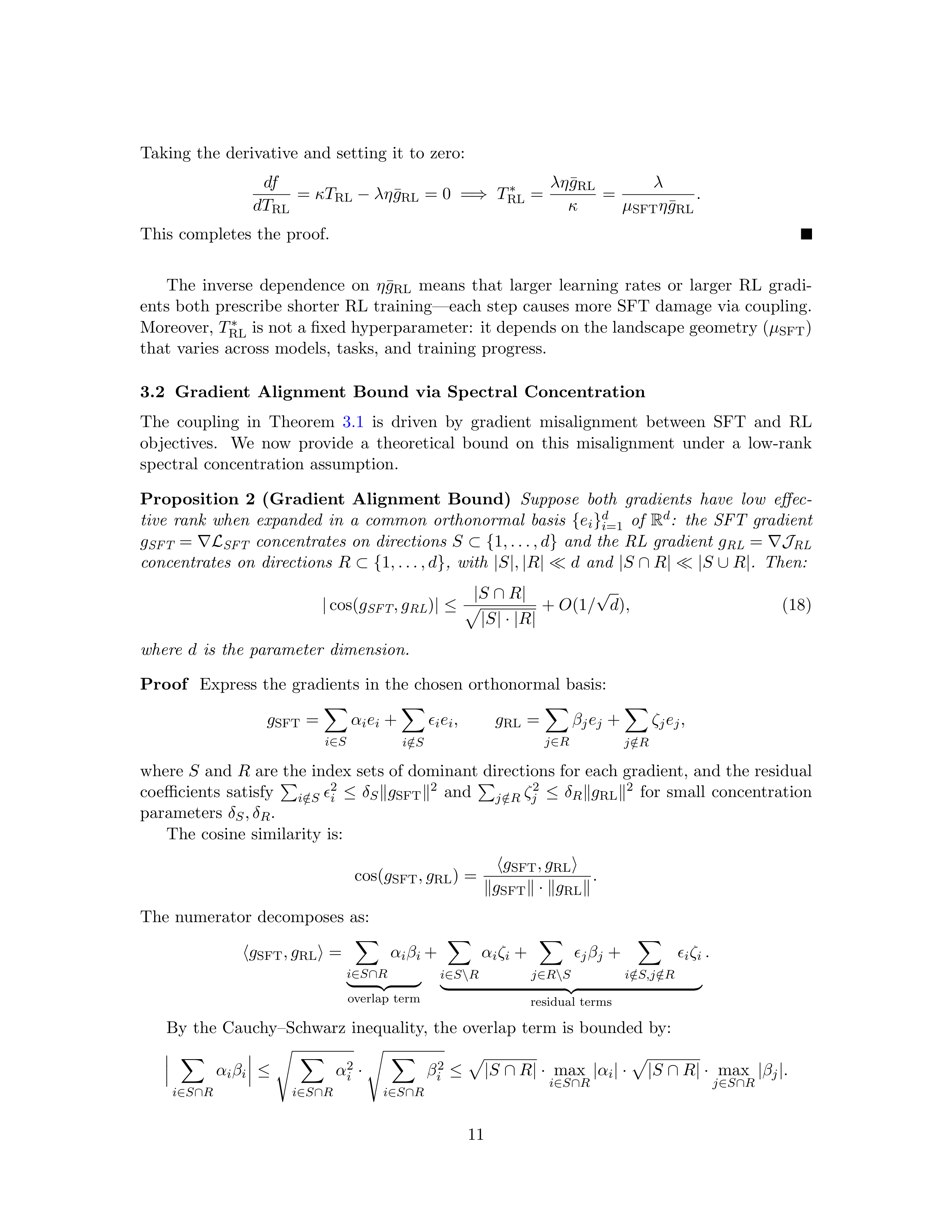
Taking
the
derivative
and
setting
it
to
zero:
df
dT
RL
=
κT
RL
−
λη
¯
g
RL
= 0
=
⇒
T
∗
RL
=
λη
¯
g
RL
κ
=
λ
µ
SFT
η
¯
g
RL
.
This
completes
the
proof.
The
inverse
dependence
on
η
¯
g
RL
means
that
larger
learning
rates
or
larger
RL
gradi-
ents
both
prescribe
shorter
RL
training—each
step
causes
more
SFT
damage
via
coupling.
Moreover,
T
∗
RL
is not a fixed hyperparameter:
it depends on the landscape geometry (
µ
SFT
)
that
varies
across
models,
tasks,
and
training
progress.
3.2
Gradient
Alignment
Bound
via
Spectral
Concentration
The
coupling
in
Theorem
3.1
is
driven
by
gradient
misalignment
between
SFT
and
RL
objectives.
We
now
provide
a
theoretical
bound
on
this
misalignment
under
a
low-rank
spectral
concentration
assumption.
Proposition
2
(Gradient
Alignment
Bound)
Suppose
both
gradients
have
low
effec-
tive
rank
when
expanded
in
a
common
orthonormal
basis
{
e
i
}
d
i
=1
of
R
d
:
the
SFT
gradient
g
SFT
=
∇L
SFT
concentrates
on
directions
S
⊂{
1
, . . . , d
}
and
the
RL
gradient
g
RL
=
∇J
RL
concentrates
on
directions
R
⊂{
1
, . . . , d
}
,
with
|
S
|
,
|
R
| ≪
d
and
|
S
∩
R
| ≪|
S
∪
R
|
.
Then:
|
cos(
g
SFT
, g
RL
)
| ≤
|
S
∩
R
|
p
|
S
| · |
R
|
+
O
(1
/
√
d
)
,
(18)
where
d
is
the
parameter
dimension.
Proof
Express
the
gradients
in
the
chosen
orthonormal
basis:
g
SFT
=
X
i
∈
S
α
i
e
i
+
X
i/
∈
S
ϵ
i
e
i
,
g
RL
=
X
j
∈
R
β
j
e
j
+
X
j /
∈
R
ζ
j
e
j
,
where
S
and
R
are the index sets of dominant directions for each gradient,
and the residual
coefficients
satisfy
P
i/
∈
S
ϵ
2
i
≤
δ
S
∥
g
SFT
∥
2
and
P
j /
∈
R
ζ
2
j
≤
δ
R
∥
g
RL
∥
2
for
small
concentration
parameters
δ
S
, δ
R
.
The
cosine
similarity
is:
cos(
g
SFT
, g
RL
) =
⟨
g
SFT
, g
RL
⟩
∥
g
SFT
∥· ∥
g
RL
∥
.
The
numerator
decomposes
as:
⟨
g
SFT
, g
RL
⟩
=
X
i
∈
S
∩
R
α
i
β
i
|
{z
}
overlap
term
+
X
i
∈
S
\
R
α
i
ζ
i
+
X
j
∈
R
\
S
ϵ
j
β
j
+
X
i/
∈
S,j /
∈
R
ϵ
i
ζ
i
|
{z
}
residual
terms
.
By
the
Cauchy–Schwarz
inequality,
the
overlap
term
is
bounded
by:
X
i
∈
S
∩
R
α
i
β
i
≤
s
X
i
∈
S
∩
R
α
2
i
·
s
X
i
∈
S
∩
R
β
2
i
≤
p
|
S
∩
R
| ·
max
i
∈
S
∩
R
|
α
i
| ·
p
|
S
∩
R
| ·
max
j
∈
S
∩
R
|
β
j
|
.
11
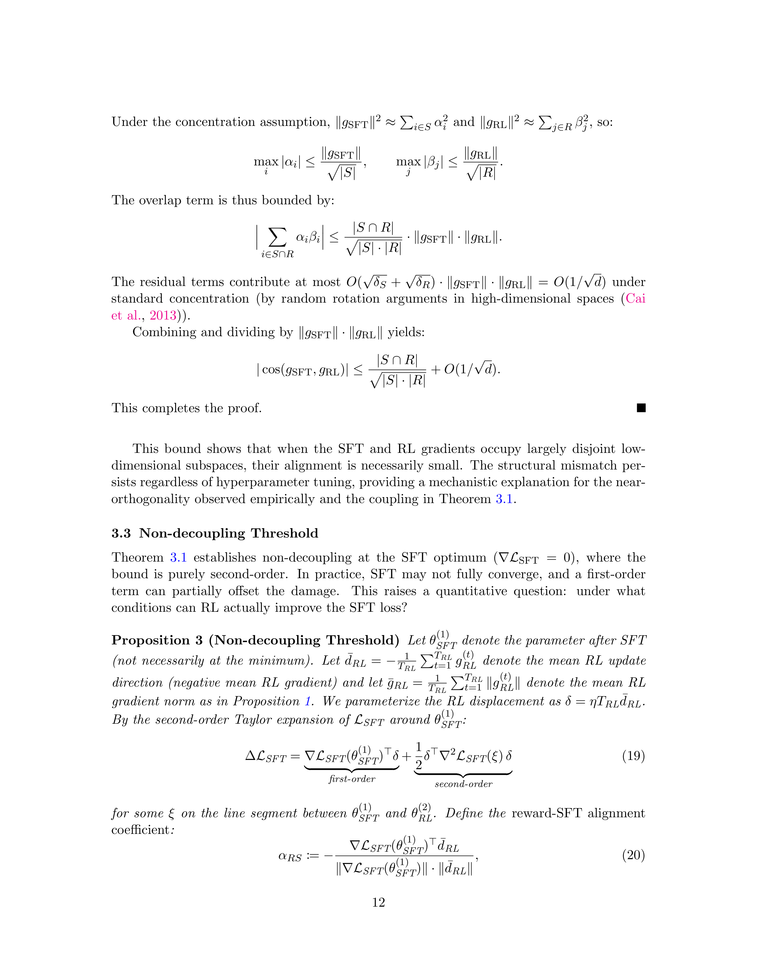
Under
the
concentration
assumption,
∥
g
SFT
∥
2
≈
P
i
∈
S
α
2
i
and
∥
g
RL
∥
2
≈
P
j
∈
R
β
2
j
,
so:
max
i
|
α
i
| ≤
∥
g
SFT
∥
p
|
S
|
,
max
j
|
β
j
| ≤
∥
g
RL
∥
p
|
R
|
.
The
overlap
term
is
thus
bounded
by:
X
i
∈
S
∩
R
α
i
β
i
≤
|
S
∩
R
|
p
|
S
| · |
R
|
· ∥
g
SFT
∥· ∥
g
RL
∥
.
The
residual
terms
contribute
at
most
O
(
√
δ
S
+
√
δ
R
)
· ∥
g
SFT
∥· ∥
g
RL
∥
=
O
(1
/
√
d
)
under
standard
concentration
(by
random
rotation
arguments
in
high-dimensional
spaces
(
Cai
et
al.
,
2013
)).
Combining
and
dividing
by
∥
g
SFT
∥· ∥
g
RL
∥
yields:
|
cos(
g
SFT
, g
RL
)
| ≤
|
S
∩
R
|
p
|
S
| · |
R
|
+
O
(1
/
√
d
)
.
This
completes
the
proof.
This
bound
shows
that
when
the
SFT
and
RL
gradients
occupy
largely
disjoint
low-
dimensional
subspaces,
their
alignment
is
necessarily
small.
The
structural
mismatch
per-
sists regardless of hyperparameter tuning, providing a mechanistic explanation for the near-
orthogonality
observed
empirically
and
the
coupling
in
Theorem
3.1
.
3.3
Non-decoupling
Threshold
Theorem
3.1
establishes
non-decoupling
at
the
SFT
optimum
(
∇L
SFT
=
0),
where
the
bound
is
purely
second-order.
In
practice,
SFT
may
not
fully
converge,
and
a
first-order
term
can
partially
offset
the
damage.
This
raises
a
quantitative
question:
under
what
conditions
can
RL
actually
improve
the
SFT
loss?
Proposition
3
(Non-decoupling
Threshold)
Let
θ
(1)
SFT
denote
the
parameter
after
SFT
(not
necessarily
at
the
minimum).
Let
¯
d
RL
=
−
1
T
RL
P
T
RL
t
=1
g
(
t
)
RL
denote
the
mean
RL
update
direction
(negative
mean
RL
gradient)
and
let
¯
g
RL
=
1
T
RL
P
T
RL
t
=1
∥
g
(
t
)
RL
∥
denote
the
mean
RL
gradient
norm
as
in
Proposition
1
.
We
parameterize
the
RL
displacement
as
δ
=
ηT
RL
¯
d
RL
.
By
the
second-order
Taylor
expansion
of
L
SFT
around
θ
(1)
SFT
:
∆
L
SFT
=
∇L
SFT
(
θ
(1)
SFT
)
⊤
δ
|
{z
}
first-order
+
1
2
δ
⊤
∇
2
L
SFT
(
ξ
)
δ
|
{z
}
second-order
(19)
for
some
ξ
on
the
line
segment
between
θ
(1)
SFT
and
θ
(2)
RL
.
Define
the
reward-SFT
alignment
coefficient
:
α
RS
:=
−
∇L
SFT
(
θ
(1)
SFT
)
⊤
¯
d
RL
∥∇L
SFT
(
θ
(1)
SFT
)
∥· ∥
¯
d
RL
∥
,
(20)
12
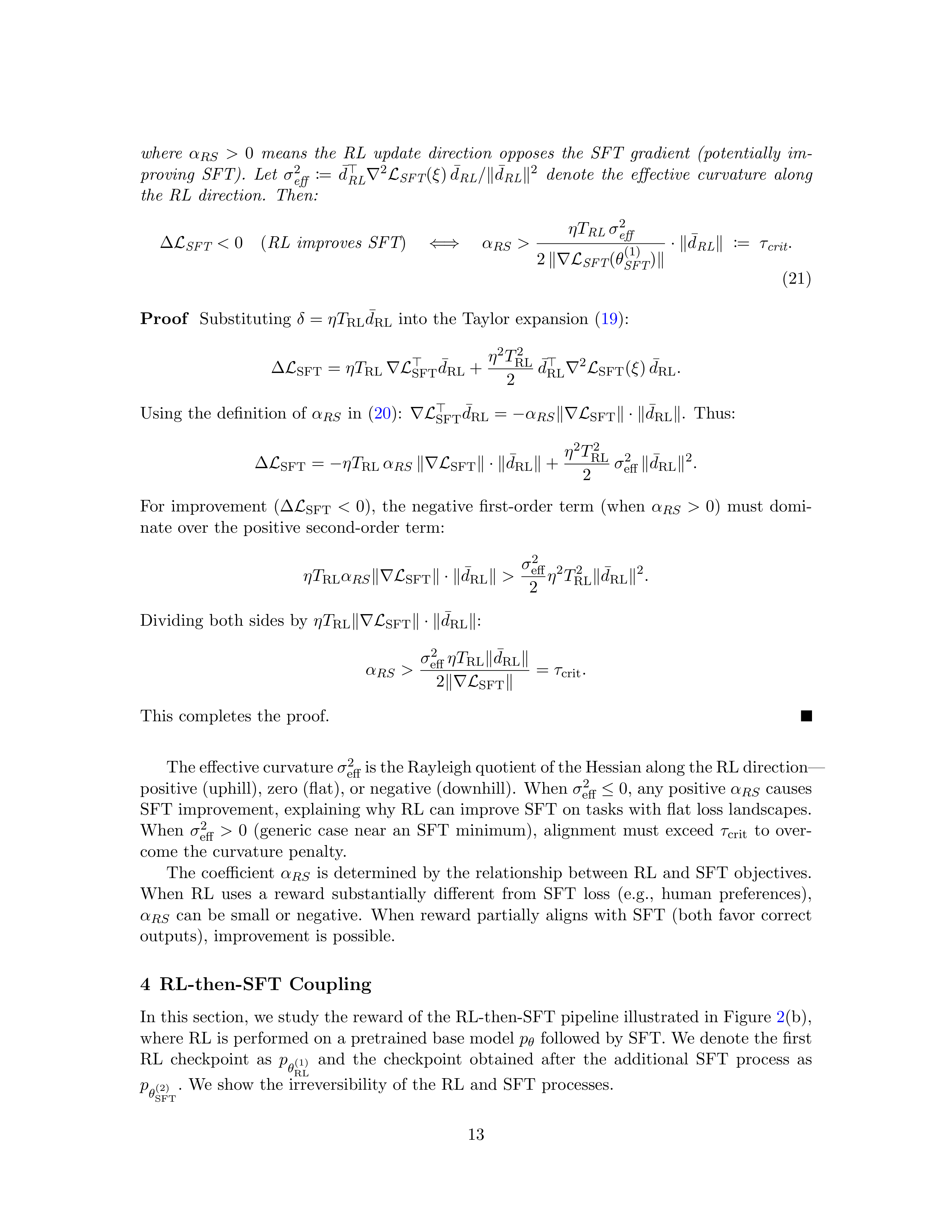
where
α
RS
>
0
means
the
RL
update
direction
opposes
the
SFT
gradient
(potentially
im-
proving
SFT).
Let
σ
2
eff
:=
¯
d
⊤
RL
∇
2
L
SFT
(
ξ
)
¯
d
RL
/
∥
¯
d
RL
∥
2
denote
the
effective
curvature
along
the
RL
direction.
Then:
∆
L
SFT
<
0
(
RL
improves
SFT
)
⇐⇒
α
RS
>
ηT
RL
σ
2
eff
2
∥∇L
SFT
(
θ
(1)
SFT
)
∥
· ∥
¯
d
RL
∥
:=
τ
crit
.
(21)
Proof
Substituting
δ
=
ηT
RL
¯
d
RL
into
the
Taylor
expansion
(
19
):
∆
L
SFT
=
ηT
RL
∇L
⊤
SFT
¯
d
RL
+
η
2
T
2
RL
2
¯
d
⊤
RL
∇
2
L
SFT
(
ξ
)
¯
d
RL
.
Using
the
definition
of
α
RS
in
(
20
):
∇L
⊤
SFT
¯
d
RL
=
−
α
RS
∥∇L
SFT
∥· ∥
¯
d
RL
∥
.
Thus:
∆
L
SFT
=
−
ηT
RL
α
RS
∥∇L
SFT
∥· ∥
¯
d
RL
∥
+
η
2
T
2
RL
2
σ
2
eff
∥
¯
d
RL
∥
2
.
For
improvement
(∆
L
SFT
<
0),
the
negative
first-order
term
(when
α
RS
>
0)
must
domi-
nate
over
the
positive
second-order
term:
ηT
RL
α
RS
∥∇L
SFT
∥· ∥
¯
d
RL
∥
>
σ
2
eff
2
η
2
T
2
RL
∥
¯
d
RL
∥
2
.
Dividing
both
sides
by
ηT
RL
∥∇L
SFT
∥· ∥
¯
d
RL
∥
:
α
RS
>
σ
2
eff
ηT
RL
∥
¯
d
RL
∥
2
∥∇L
SFT
∥
=
τ
crit
.
This
completes
the
proof.
The effective curvature
σ
2
eff
is the Rayleigh quotient of the Hessian along the RL direction—
positive (uphill), zero (flat), or negative (downhill).
When
σ
2
eff
≤
0, any positive
α
RS
causes
SFT
improvement,
explaining
why
RL
can
improve
SFT
on
tasks
with
flat
loss
landscapes.
When
σ
2
eff
>
0
(generic
case
near
an
SFT
minimum),
alignment
must
exceed
τ
crit
to
over-
come
the
curvature
penalty.
The
coefficient
α
RS
is
determined
by
the
relationship
between
RL
and
SFT
objectives.
When
RL
uses
a
reward
substantially
different
from
SFT
loss
(e.g.,
human
preferences),
α
RS
can
be
small
or
negative.
When
reward
partially
aligns
with
SFT
(both
favor
correct
outputs),
improvement
is
possible.
4
RL-then-SFT
Coupling
In this section,
we study the reward of the RL-then-SFT pipeline illustrated in Figure
2
(b),
where
RL
is
performed
on
a
pretrained
base
model
p
θ
followed
by
SFT.
We
denote
the
first
RL
checkpoint
as
p
θ
(1)
RL
and
the
checkpoint
obtained
after
the
additional
SFT
process
as
p
θ
(2)
SFT
.
We
show
the
irreversibility
of
the
RL
and
SFT
processes.
13
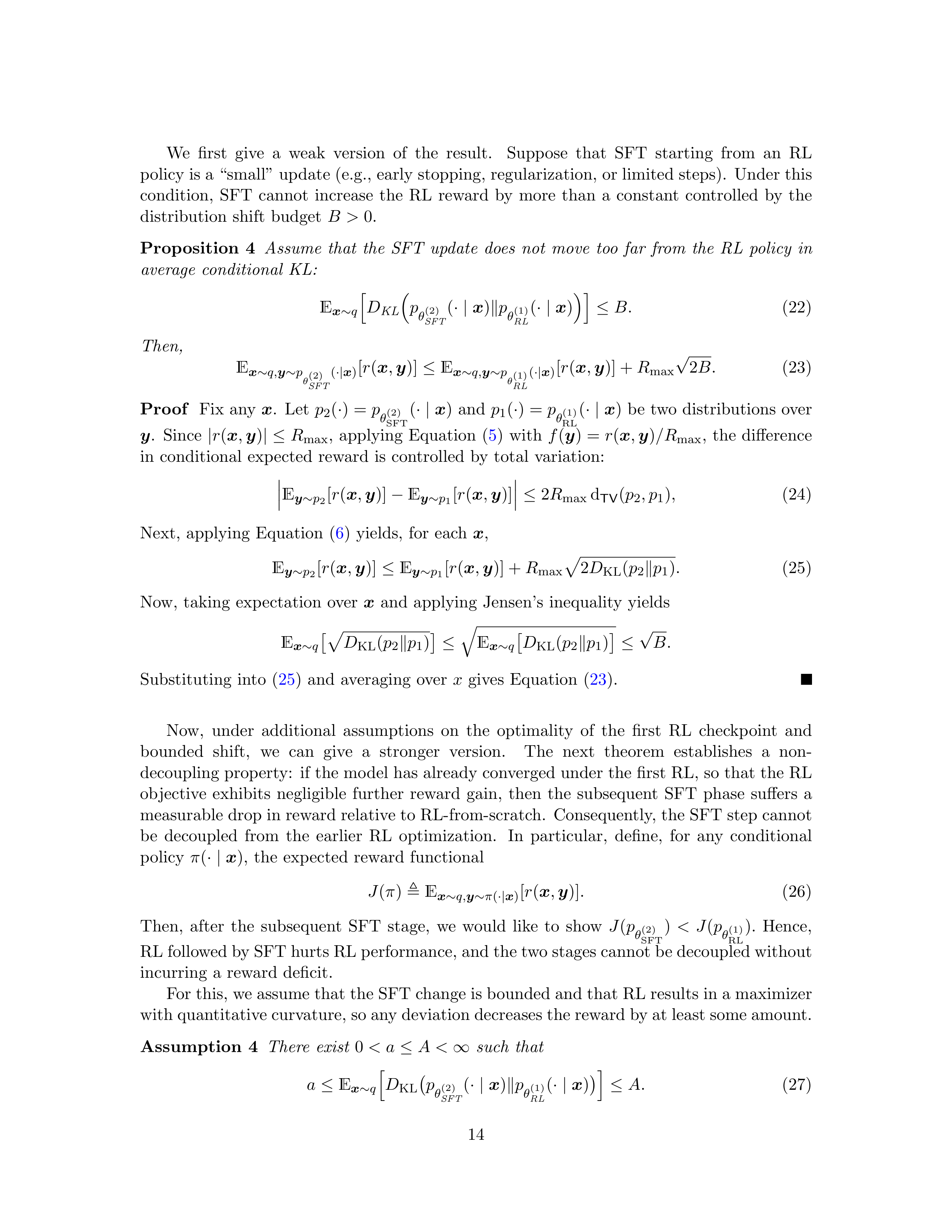
We
first
give
a
weak
version
of
the
result.
Suppose
that
SFT
starting
from
an
RL
policy is a “small” update (e.g., early stopping, regularization, or limited steps).
Under this
condition,
SFT
cannot
increase
the
RL
reward
by
more
than
a
constant
controlled
by
the
distribution
shift
budget
B
>
0.
Proposition
4
Assume
that
the
SFT
update
does
not
move
too
far
from
the
RL
policy
in
average
conditional
KL:
E
x
∼
q
h
D
KL
p
θ
(2)
SFT
(
· |
x
)
∥
p
θ
(1)
RL
(
· |
x
)
i
≤
B.
(22)
Then,
E
x
∼
q,
y
∼
p
θ
(2)
SFT
(
·|
x
)
[
r
(
x
,
y
)]
≤
E
x
∼
q,
y
∼
p
θ
(1)
RL
(
·|
x
)
[
r
(
x
,
y
)] +
R
max
√
2
B.
(23)
Proof
Fix
any
x
.
Let
p
2
(
·
) =
p
θ
(2)
SFT
(
· |
x
)
and
p
1
(
·
) =
p
θ
(1)
RL
(
· |
x
)
be
two
distributions
over
y
.
Since
|
r
(
x
,
y
)
| ≤
R
max
,
applying
Equation
(
5
)
with
f
(
y
) =
r
(
x
,
y
)
/R
max
,
the
difference
in
conditional
expected
reward
is
controlled
by
total
variation:
E
y
∼
p
2
[
r
(
x
,
y
)]
−
E
y
∼
p
1
[
r
(
x
,
y
)]
≤
2
R
max
d
TV
(
p
2
, p
1
)
,
(24)
Next,
applying
Equation
(
6
)
yields,
for
each
x
,
E
y
∼
p
2
[
r
(
x
,
y
)]
≤
E
y
∼
p
1
[
r
(
x
,
y
)] +
R
max
p
2
D
KL
(
p
2
∥
p
1
)
.
(25)
Now,
taking
expectation
over
x
and
applying
Jensen’s
inequality
yields
E
x
∼
q
p
D
KL
(
p
2
∥
p
1
)
≤
q
E
x
∼
q
D
KL
(
p
2
∥
p
1
)
≤
√
B.
Substituting
into
(
25
)
and
averaging
over
x
gives
Equation
(
23
).
Now,
under
additional
assumptions
on
the
optimality
of
the
first
RL
checkpoint
and
bounded
shift,
we
can
give
a
stronger
version.
The
next
theorem
establishes
a
non-
decoupling property:
if the model has already converged under the first RL, so that the RL
objective
exhibits
negligible
further
reward
gain,
then
the
subsequent
SFT
phase
suffers
a
measurable drop in reward relative to RL-from-scratch.
Consequently, the SFT step cannot
be
decoupled
from
the
earlier
RL
optimization.
In
particular,
define,
for
any
conditional
policy
π
(
· |
x
),
the
expected
reward
functional
J
(
π
)
≜
E
x
∼
q,
y
∼
π
(
·|
x
)
[
r
(
x
,
y
)]
.
(26)
Then,
after
the
subsequent
SFT
stage,
we
would
like
to
show
J
(
p
θ
(2)
SFT
)
<
J
(
p
θ
(1)
RL
)
.
Hence,
RL followed by SFT hurts RL performance, and the two stages cannot be decoupled without
incurring
a
reward
deficit.
For this, we assume that the SFT change is bounded and that RL results in a maximizer
with quantitative curvature, so any deviation decreases the reward by at least some amount.
Assumption
4
There
exist
0
< a
≤
A <
∞
such
that
a
≤
E
x
∼
q
h
D
KL
p
θ
(2)
SFT
(
· |
x
)
∥
p
θ
(1)
RL
(
· |
x
)
i
≤
A.
(27)
14
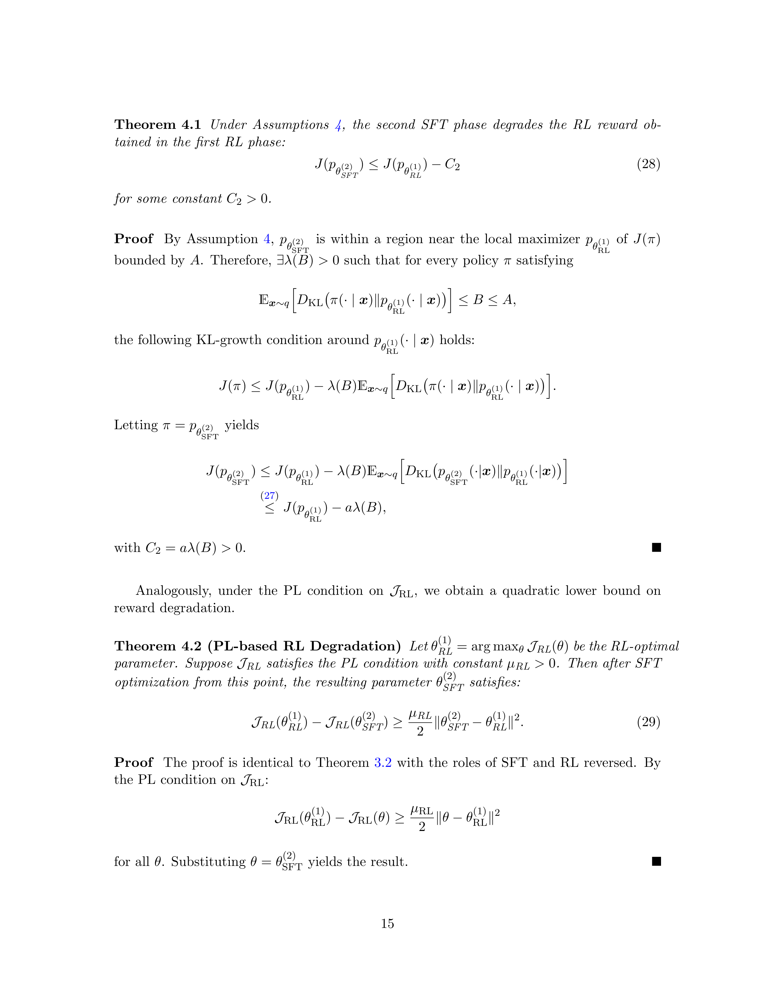
Theorem
4.1
Under
Assumptions
4
,
the
second
SFT
phase
degrades
the
RL
reward
ob-
tained
in
the
first
RL
phase:
J
(
p
θ
(2)
SFT
)
≤
J
(
p
θ
(1)
RL
)
−
C
2
(28)
for
some
constant
C
2
>
0
.
Proof
By
Assumption
4
,
p
θ
(2)
SFT
is
within
a
region
near
the
local
maximizer
p
θ
(1)
RL
of
J
(
π
)
bounded
by
A
.
Therefore,
∃
λ
(
B
)
>
0
such
that
for
every
policy
π
satisfying
E
x
∼
q
h
D
KL
π
(
· |
x
)
∥
p
θ
(1)
RL
(
· |
x
)
i
≤
B
≤
A,
the
following
KL-growth
condition
around
p
θ
(1)
RL
(
· |
x
)
holds:
J
(
π
)
≤
J
(
p
θ
(1)
RL
)
−
λ
(
B
)
E
x
∼
q
h
D
KL
π
(
· |
x
)
∥
p
θ
(1)
RL
(
· |
x
)
i
.
Letting
π
=
p
θ
(2)
SFT
yields
J
(
p
θ
(2)
SFT
)
≤
J
(
p
θ
(1)
RL
)
−
λ
(
B
)
E
x
∼
q
h
D
KL
p
θ
(2)
SFT
(
·|
x
)
∥
p
θ
(1)
RL
(
·|
x
)
i
(
27
)
≤
J
(
p
θ
(1)
RL
)
−
aλ
(
B
)
,
with
C
2
=
aλ
(
B
)
>
0
.
Analogously,
under
the
PL
condition
on
J
RL
,
we
obtain
a
quadratic
lower
bound
on
reward
degradation.
Theorem
4.2
(PL-based
RL
Degradation)
Let
θ
(1)
RL
= arg max
θ
J
RL
(
θ
)
be the RL-optimal
parameter.
Suppose
J
RL
satisfies
the
PL
condition
with
constant
µ
RL
>
0
.
Then
after
SFT
optimization
from
this
point,
the
resulting
parameter
θ
(2)
SFT
satisfies:
J
RL
(
θ
(1)
RL
)
−J
RL
(
θ
(2)
SFT
)
≥
µ
RL
2
∥
θ
(2)
SFT
−
θ
(1)
RL
∥
2
.
(29)
Proof
The
proof
is
identical
to
Theorem
3.2
with
the
roles
of
SFT
and
RL
reversed.
By
the
PL
condition
on
J
RL
:
J
RL
(
θ
(1)
RL
)
−J
RL
(
θ
)
≥
µ
RL
2
∥
θ
−
θ
(1)
RL
∥
2
for
all
θ
.
Substituting
θ
=
θ
(2)
SFT
yields
the
result.
15
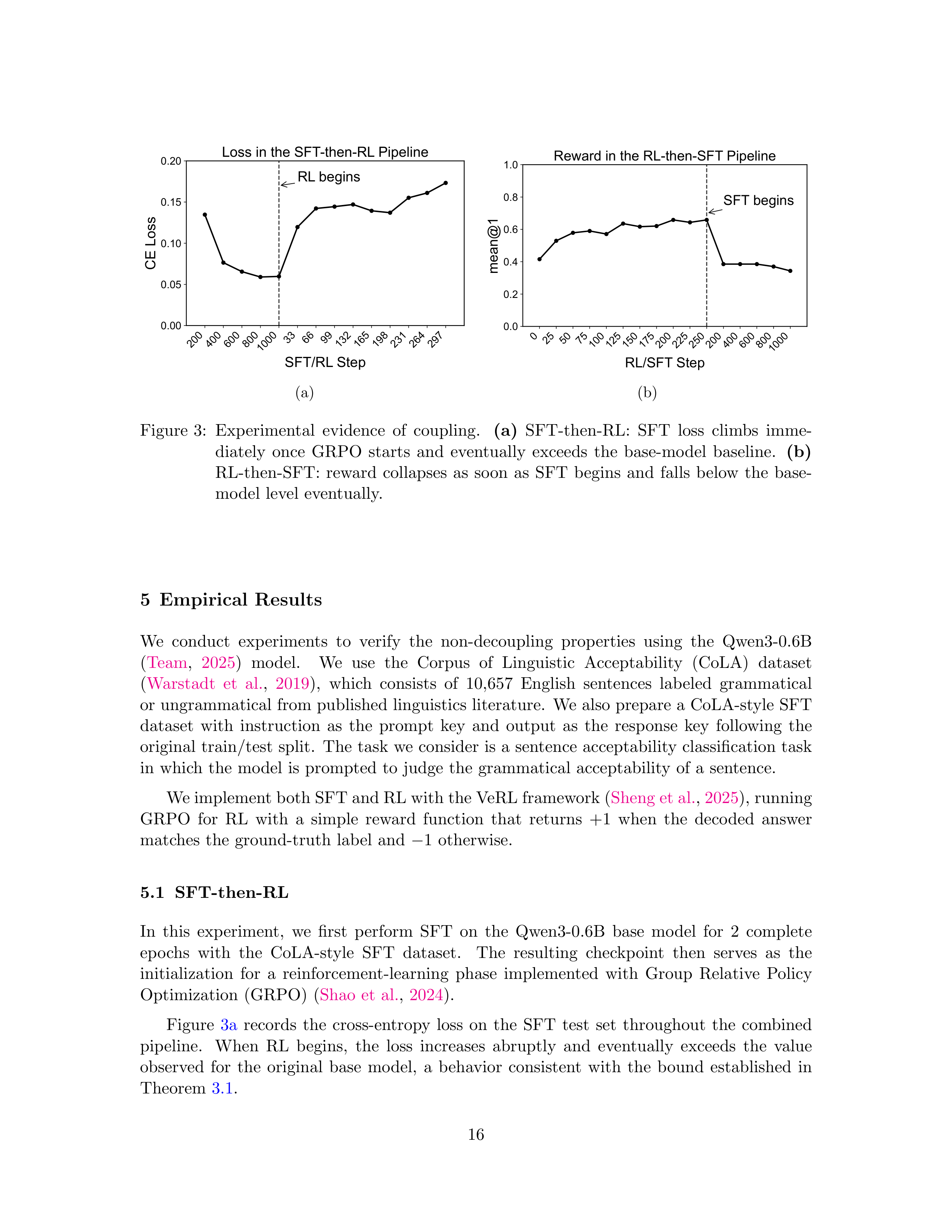
200
400
600
800
1000
33
66
99
132
165
198
231
264
297
SFT/RL Step
0.00
0.05
0.10
0.15
0.20
CE Loss
RL begins
Loss in the SFT-then-RL Pipeline
(a)
0
25
50
75
100
125
150
175
200
225
250
200
400
600
800
1000
RL/SFT Step
0.0
0.2
0.4
0.6
0.8
1.0
mean@1
SFT begins
Reward in the RL-then-SFT Pipeline
(b)
Figure
3:
Experimental
evidence
of
coupling.
(a)
SFT-then-RL:
SFT
loss
climbs
imme-
diately
once
GRPO
starts
and
eventually
exceeds
the
base-model
baseline.
(b)
RL-then-SFT:
reward
collapses
as
soon
as
SFT
begins
and
falls
below
the
base-
model
level
eventually.
5
Empirical
Results
We
conduct
experiments
to
verify
the
non-decoupling
properties
using
the
Qwen3-0.6B
(
Team
,
2025
)
model.
We
use
the
Corpus
of
Linguistic
Acceptability
(CoLA)
dataset
(
Warstadt
et
al.
,
2019
),
which
consists
of
10,657
English
sentences
labeled
grammatical
or
ungrammatical
from
published
linguistics
literature.
We
also
prepare
a
CoLA-style
SFT
dataset
with
instruction
as
the
prompt
key
and
output
as
the
response
key
following
the
original
train/test
split.
The
task
we
consider
is
a
sentence
acceptability
classification
task
in
which
the
model
is
prompted
to
judge
the
grammatical
acceptability
of
a
sentence.
We implement both SFT and RL with the VeRL framework (
Sheng et al.
,
2025
), running
GRPO
for
RL
with
a
simple
reward
function
that
returns
+1
when
the
decoded
answer
matches
the
ground-truth
label
and
−
1
otherwise.
5.1
SFT-then-RL
In
this
experiment,
we
first
perform
SFT
on
the
Qwen3-0.6B
base
model
for
2
complete
epochs
with
the
CoLA-style
SFT
dataset.
The
resulting
checkpoint
then
serves
as
the
initialization
for
a
reinforcement-learning
phase
implemented
with
Group
Relative
Policy
Optimization
(GRPO)
(
Shao
et
al.
,
2024
).
Figure
3a
records
the
cross-entropy
loss
on
the
SFT
test
set
throughout
the
combined
pipeline.
When
RL
begins,
the
loss
increases
abruptly
and
eventually
exceeds
the
value
observed
for
the
original
base
model,
a
behavior
consistent
with
the
bound
established
in
Theorem
3.1
.
16
5.2
RL-then-SFT
In
this
experiment,
we
first
perform
RL
with
GRPO
on
the
Qwen3-0.6B
base
model.
Once
the
RL
phase
converges,
we
use
that
model
as
the
initialization
for
an
SFT
phase
for
2
complete
epochs
on
the
same
CoLA-style
SFT
data.
We
evaluate
the
rewards
using
the
same
settings
as
the
validation
rollout
from
the
RL
stage
(
temperature
=
0
.
6
,
top
p
=
0
.
95).
The
reward
function
is
strict
on
the
format
in
RL
training.
However,
the
SFT
model
can
output
labels
in
slightly
different
formats,
therefore
assigning
−
1
even
if
the
answer
is
semantically
correct.
To
reduce
the
format
sensitivity
only
in
evaluation,
we
used
a
robust
evaluation
which
keeps
the
same
scoring
rule
(+1
for
correct
label,
−
1
otherwise)
while
scanning
the
whole
output
for
“acceptable”
/
“unacceptable”
and
use
the
last
occurrence.
We
report
the
mean
@
1
reward
(one
output
per
prompt)
for
the
entire
RL-then-SFT
pipeline
on
the
RL
test
set
in
Figure
3b
.
The
SFT
steps
overwrite
the
RL-tuned
behavior
and
hurt
label
accuracy,
consistent
with
Theorem
4.1
,
and
a
sharp
drop
in
reward
can
be
observed.
In
particular,
the
base
model
(step
0),
under
robust
evaluation,
has
mean
@
1
≈
0
.
385,
i.e.
approximately
69.5%
accuracy.
The
final
SFT
checkpoint
has
mean
@
1
≈
0
.
343
,
i.e.,
approximately
67.2%
accuracy,
even
lower
than
the
base
model.
6
Conclusion
Our
analysis
of
the
two
canonical
post-training
pipelines
shows
that
supervised
fine-tuning
and
reinforcement
learning
are
inherently
coupled:
whichever
order
is
adopted,
the
second
stage
degrades
the
performance
achieved
by
the
first.
We
establish
this
through
comple-
mentary
theoretical
lenses:
distributional
analysis
via
KL
divergence
gives
nonnegativity
of
the
degradation,
while
the
PL
condition
yields
explicit
quadratic
bounds
that
scale
with
parameter
displacement.
Our
results
further
reveal
that:
(i)
the
coupling
damage
grows
quadratically
with
RL
duration
whereas
reward
improvement
grows
at
most
linearly,
im-
plying
the
existence
of
an
optimal
stopping
point;
(ii)
gradient
near-orthogonality
between
SFT
and
RL
objectives
is
a
consequence
of
spectral
concentration
in
different
parameter
subspaces;
and
(iii)
the
non-decoupling
threshold
identifies
precisely
when
RL
can
(or
can-
not)
improve
SFT
performance.
Empirical
results
on
the
Qwen3-0.6B
model
corroborate
these
guarantees,
revealing
abrupt
degradation
in
either
cross-entropy
or
reward
when
the
transition
occurs.
We
hope
that
these
theoretical
insights
will
inform
the
development
of
new
training
strategies,
such
as
gradient
surgery,
landscape-aware
scheduling,
or
joint
optimization,
that
better
balance
memorization
and
generalization
to
build
more
capable
models.
Recognizing
non-decoupling
could
reduce
post-training
compute
by
eliminating
destructive
RL
steps,
lowering
both
carbon
emissions
and
development
barriers.
17
References
S.
Aich.
From
sublinear
to
linear:
Fast
convergence
in
deep
networks
via
locally
Polyak-
lojasiewicz
regions.
arXiv
preprint
arXiv:2507.21429
,
2025.
S.
N.
Akter,
S.
Prabhumoye,
E.
Nyberg,
M.
Patwary,
M.
Shoeybi,
Y.
Choi,
and
B.
Catan-
zaro.
Front-loading
reasoning:
The
synergy
between
pretraining
and
post-training
data.
arXiv
preprint
arXiv:2510.03264
,
2025.
Y. Bai, A. Jones, K. Ndousse, A. Askell, A. Chen, N. DasSarma, D. Drain, S. Fort, D. Gan-
guli,
T.
Henighan,
et
al.
Training
a
helpful
and
harmless
assistant
with
reinforcement
learning
from
human
feedback.
arXiv
preprint
arXiv:2204.05862
,
2022.
R.
A.
Bradley
and
M.
E.
Terry.
Rank
analysis
of
incomplete
block
designs:
I.
the
method
of
paired
comparisons.
Biometrika
,
39(3/4):324–345,
1952.
T.
Cai,
J.
Fan,
and
T.
Jiang.
Distributions
of
angles
in
random
packing
on
spheres.
The
Journal
of
Machine
Learning
Research
,
14(1):1837–1864,
2013.
J. Chen, T. Yu, H. Bai, L. Yao, J. Wu, K. Li, F. Mi, C. Tao, L. Zhu, M. Zhang, X. Li, L. Hou,
L. Shang, and Q. Liu.
The synergy dilemma of long-CoT SFT and RL: Investigating post-
training
techniques
for
reasoning
VLMs.
arXiv
preprint
arXiv:2507.07562
,
2025a.
L. Chen, X. Han, L. Shen, J. Bai, and K.-F. Wong.
Beyond two-stage training:
Cooperative
SFT
and
RL
for
LLM
reasoning.
arXiv
preprint
arXiv:2509.06948
,
2025b.
P.
F.
Christiano,
J.
Leike,
T.
Brown,
M.
Martic,
S.
Legg,
and
D.
Amodei.
Deep
rein-
forcement
learning
from
human
preferences.
Advances
in
Neural
Information
Processing
Systems
,
30,
2017.
T. Chu,
Y. Zhai,
J. Yang,
S. Tong,
S. Xie,
D. Schuurmans,
Q. V. Le,
S. Levine,
and Y. Ma.
SFT memorizes, RL generalizes:
A comparative study of foundation model post-training.
arXiv
preprint
arXiv:2501.17161
,
2025.
D.
Guo,
D.
Yang,
H.
Zhang,
J.
Song,
R.
Zhang,
R.
Xu,
Q.
Zhu,
S.
Ma,
P.
Wang,
X.
Bi,
et al.
Deepseek-r1:
Incentivizing reasoning capability in LLMs via reinforcement learning.
arXiv
preprint
arXiv:2501.12948
,
2025.
B. He, Z. Qu, Z. Liu, Y. Chen, Y. Zuo, C. Qian, K. Zhang, W. Chen, C. Xiao, G. Cui, et al.
JustRL:
Scaling
a
1.5b
LLM
with
a
simple
RL
recipe.
arXiv
preprint
arXiv:2512.16649
,
2025.
M.
Huan,
Y.
Li,
T.
Zheng,
X.
Xu,
S.
Kim,
M.
Du,
R.
Poovendran,
G.
Neubig,
and
X.
Yue.
Does math reasoning improve general LLM capabilities?
understanding transferability of
LLM
reasoning.
arXiv
preprint
arXiv:2507.00432
,
2025.
H. Karimi, J. Nutini, and M. Schmidt. Linear convergence of gradient and proximal-gradient
methods
under
the
Polyak-
lojasiewicz
condition.
In
Joint
European
Conference
on
Ma-
chine
Learning
and
Knowledge
Discovery
in
Databases
,
Cham,
2016.
Springer
Interna-
tional
Publishing.
18
N.
Lambert,
J.
Morrison,
V.
Pyatkin,
S.
Huang,
H.
Ivison,
F.
Brahman,
L.
J.
V.
Miranda,
A.
Liu,
N.
Dziri,
S.
Lyu,
Y.
Gu,
S.
Malik,
V.
Graf,
J.
D.
Hwang,
J.
Yang,
R.
L.
Bras,
O.
Tafjord,
C.
Wilhelm,
L.
Soldaini,
N.
A.
Smith,
Y.
Wang,
P.
Dasigi,
and
H.
Ha-
jishirzi.
Tulu
3:
Pushing
frontiers
in
open
language
model
post-training.
arXiv
preprint
arXiv:2411.15124
,
2025.
Z.
Liu,
Z.
Yang,
Y.
Chen,
C.
Lee,
M.
Shoeybi,
B.
Catanzaro,
and
W.
Ping.
AceReason-
Nemotron 1.1:
Advancing math and code reasoning through SFT and RL synergy.
arXiv
preprint
arXiv:2506.13284
,
2025.
X.
Niu,
B.
Bai,
L.
Deng,
and
W.
Han.
Beyond
scaling
laws:
Understanding
transformer
performance
with
associative
memory.
arXiv
preprint
arXiv:2405.08707
,
2024.
X.
Niu,
B.
Bai,
N.
Guo,
W.
Zhang,
and
W.
Han.
Rate–distortion–perception
trade-off
in
information
theory,
generative
models,
and
intelligent
communications.
Entropy
,
27(4):
373,
2025.
L. Ouyang, J. Wu, X. Jiang, D. Almeida, C. Wainwright, P. Mishkin, C. Zhang, S. Agarwal,
K.
Slama,
A.
Ray,
et
al.
Training
language
models
to
follow
instructions
with
human
feedback.
Advances
in
Neural
Information
Processing
Systems
,
35:27730–27744,
2022.
X.
B.
Peng,
A.
Kumar,
G.
Zhang,
and
S.
Levine.
Advantage-weighted
regression:
Simple
and
scalable
off-policy
reinforcement
learning.
arXiv
preprint
arXiv:1910.00177
,
2019.
M.
S.
Pinsker.
Information
and
information
stability
of
random
variables
and
processes.
Holden-Day
,
1964.
B.
T.
Polyak.
Gradient
methods
for
the
minimisation
of
functionals.
USSR
Computational
Mathematics
and
Mathematical
Physics
,
3(4):864–878,
1963.
N.
Razin,
Z.
Wang,
H.
Strauss,
S.
Wei,
J.
D.
Lee,
and
S.
Arora.
What
makes
a
reward
model
a
good
teacher?
an
optimization
perspective.
arXiv
preprint
arXiv:2503.15477
,
2025.
J.
Schulman,
F.
Wolski,
P.
Dhariwal,
A.
Radford,
and
O.
Klimov.
Proximal
policy
opti-
mization
algorithms.
arXiv
preprint
arXiv:1707.06347
,
2017.
Z.
Shao,
P.
Wang,
Q.
Zhu,
R.
Xu,
J.
Song,
X.
Bi,
H.
Zhang,
M.
Zhang,
Y.
Li,
Y.
Wu,
et
al.
Deepseekmath:
Pushing
the
limits
of
mathematical
reasoning
in
open
language
models.
arXiv
preprint
arXiv:2402.03300
,
2024.
G.
Sheng,
C.
Zhang,
Z.
Ye,
X.
Wu,
W.
Zhang,
R.
Zhang,
Y.
Peng,
H.
Lin,
and
C.
Wu.
Hybridflow:
A
flexible
and
efficient
rlhf
framework.
In
Proceedings
of
the
Twentieth
European
Conference
on
Computer
Systems
,
EuroSys
’25,
page
1279–1297,
New
York,
NY,
USA,
2025.
Association
for
Computing
Machinery.
ISBN
9798400711961.
Q.
Team.
Qwen3
technical
report,
2025.
URL
https://arxiv.org/abs/2505.09388
.
B. Wang, C. Lee, N. Lee, S.-C. Lin, W. Dai, Y. Chen, Y. Chen, Z. Yang, Z. Liu, M. Shoeybi,
et
al.
Nemotron-cascade:
Scaling
cascaded
reinforcement
learning
for
general-purpose
reasoning
models.
arXiv
preprint
arXiv:2512.13607
,
2025.
19
A. Warstadt, A. Singh, and S. R. Bowman.
Neural network acceptability judgments.
Trans-
actions
of
the
Association
for
Computational
Linguistics
,
7:625–641,
2019.
J. Yan, Y. Li,
Z. Hu,
Z. Wang,
G. Cui,
X. Qu,
Y. Cheng,
and Y. Zhang.
Learning to reason
under off-policy guidance.
In
The Thirty-ninth Annual Conference on Neural Information
Processing
Systems
,
2025.
Q.
Yu,
Z.
Zhang,
R.
Zhu,
Y.
Yuan,
X.
Zuo,
Y.
Yue,
W.
Dai,
T.
Fan,
G.
Liu,
L.
Liu,
et
al.
Dapo:
An
open-source
llm
reinforcement
learning
system
at
scale.
arXiv
preprint
arXiv:2503.14476
,
2025.
T.
Yu,
S.
Kumar,
A.
Gupta,
S.
Levine,
K.
Hausman,
and
C.
Finn.
Gradient
surgery
for
multi-task
learning.
Advances
in
Neural
Information
Processing
Systems
,
33:5824–5836,
2020.
Y.
Yue,
Y.
Yuan,
Q.
Yu,
X.
Zuo,
R.
Zhu,
W.
Xu,
J.
Chen,
C.
Wang,
T.
Fan,
Z.
Du,
et
al.
Vapo:
Efficient
and
reliable
reinforcement
learning
for
advanced
reasoning
tasks.
arXiv
preprint
arXiv:2504.05118
,
2025.
C.
Zhang,
S.
Bengio,
M.
Hardt,
B.
Recht,
and
O.
Vinyals.
Understanding
deep
learning
requires
rethinking
generalization.
arXiv
preprint
arXiv:1611.03530
,
2016.
D.
M.
Ziegler,
N.
Stiennon,
J.
Wu,
T.
B.
Brown,
A.
Radford,
D.
Amodei,
P.
Christiano,
and
G.
Irving.
Fine-tuning
language
models
from
human
preferences.
arXiv
preprint
arXiv:1909.08593
,
2019.
20