
Deep Unsupervised Learning using
Nonequilibrium Thermodynamics
Jascha Sohl-Dickstein
JASCHA
@
STANFORD
.
EDU
Stanford University
Eric A. Weiss
EAWEISS
@
BERKELEY
.
EDU
University of California, Berkeley
Niru Maheswaranathan
NIRUM
@
STANFORD
.
EDU
Stanford University
Surya Ganguli
SGANGULI
@
STANFORD
.
EDU
Stanford University
Abstract
A
central
problem
in
machine
learning
involves
modeling
complex
data-sets
using
highly
flexi-
ble families of probability distributions in which
learning,
sampling,
inference,
and
evaluation
are still analytically or computationally tractable.
Here,
we
develop
an
approach
that
simultane-
ously
achieves
both
flexibility
and
tractability.
The
essential
idea,
inspired
by
non-equilibrium
statistical physics, is to systematically and slowly
destroy
structure
in
a
data
distribution
through
an
iterative
forward
diffusion
process.
We
then
learn
a
reverse
diffusion
process
that
restores
structure
in
data,
yielding
a
highly
flexible
and
tractable
generative
model
of
the
data.
This
ap-
proach
allows
us
to
rapidly
learn,
sample
from,
and
evaluate
probabilities
in
deep
generative
models
with
thousands
of
layers
or
time
steps,
as
well
as
to
compute
conditional
and
posterior
probabilities under the learned model.
We addi-
tionally
release
an
open
source
reference
imple-
mentation of the algorithm.
1. Introduction
Historically, probabilistic models suffer from a tradeoff be-
tween
two
conflicting
objectives:
tractability
and
flexibil-
ity
.
Models that are
tractable
can be analytically evaluated
and easily fit to data (e.g. a Gaussian or Laplace). However,
Proceedings
of
the
32
nd
International
Conference
on
Machine
Learning
, Lille, France, 2015.
JMLR: W&CP volume 37.
Copy-
right 2015 by the author(s).
these
models
are
unable
to
aptly
describe
structure
in
rich
datasets.
On the other hand, models that are
flexible
can be
molded
to
fit
structure
in
arbitrary
data.
For
example,
we
can define models in terms of any (non-negative) function
φ
(
x
)
yielding the flexible distribution
p
(
x
) =
φ
(
x
)
Z
, where
Z
is
a
normalization
constant.
However,
computing
this
normalization constant is generally intractable. Evaluating,
training, or drawing samples from such flexible models typ-
ically requires a very expensive Monte Carlo process.
A
variety
of
analytic
approximations
exist
which
amelio-
rate,
but
do
not
remove,
this
tradeoff–for
instance
mean
field
theory
and
its
expansions
(
T
,
1982
;
Tanaka
,
1998
),
variational
Bayes
(
Jordan
et
al.
,
1999
),
contrastive
diver-
gence (
Welling & Hinton
,
2002
;
Hinton
,
2002
),
minimum
probability flow (
Sohl-Dickstein et al.
,
2011b
;
a
), minimum
KL
contraction
(
Lyu
,
2011
),
proper
scoring
rules
(
Gneit-
ing
&
Raftery
,
2007
;
Parry
et
al.
,
2012
),
score
matching
(
Hyv¨arinen
,
2005
), pseudolikelihood (
Besag
,
1975
), loopy
belief propagation (
Murphy et al.
,
1999
), and many, many
more.
Non-parametric
methods
(
Gershman
&
Blei
,
2012
)
can also be very effective
1
.
1.1. Diffusion probabilistic models
We present a novel way to define probabilistic models that
allows:
1.
extreme flexibility in model structure,
2.
exact sampling,
1
Non-parametric
methods
can
be
seen
as
transitioning
smoothly
between
tractable
and
flexible
models.
For
instance,
a
non-parametric
Gaussian
mixture
model
will
represent
a
small
amount of data using a single Gaussian, but may represent infinite
data as a mixture of an infinite number of Gaussians.
arXiv:1503.03585v8 [cs.LG] 18 Nov 2015
Deep Unsupervised Learning using Nonequilibrium Thermodynamics
3.
easy multiplication with other distributions, e.g.
in or-
der to compute a posterior, and
4.
the model
log
likelihood,
and
the
probability
of indi-
vidual states, to be cheaply evaluated.
Our method uses a Markov chain to gradually convert one
distribution
into
another,
an
idea
used
in
non-equilibrium
statistical
physics
(
Jarzynski
,
1997
)
and
sequential
Monte
Carlo
(
Neal
,
2001
).
We
build
a
generative
Markov
chain
which
converts
a
simple
known
distribution
(e.g.
a
Gaus-
sian) into a target (data) distribution using a diffusion pro-
cess.
Rather than use this Markov chain to approximately
evaluate a model which has been otherwise defined, we ex-
plicitly define the probabilistic model as the endpoint of the
Markov chain. Since each step in the diffusion chain has an
analytically evaluable probability, the full chain can also be
analytically evaluated.
Learning in this framework involves estimating small per-
turbations to a diffusion process.
Estimating small pertur-
bations is more tractable than explicitly describing the full
distribution
with
a
single,
non-analytically-normalizable,
potential
function.
Furthermore,
since
a
diffusion
process
exists
for
any
smooth
target
distribution,
this
method
can
capture data distributions of arbitrary form.
We
demonstrate
the
utility
of
these
diffusion
probabilistic
models
by
training
high
log
likelihood
models
for
a
two-
dimensional swiss roll, binary sequence, handwritten digit
(MNIST), and several natural image (CIFAR-10, bark, and
dead leaves) datasets.
1.2. Relationship to other work
The
wake-sleep
algorithm
(
Hinton
,
1995
;
Dayan
et
al.
,
1995
)
introduced
the
idea
of
training
inference
and
gen-
erative
probabilistic
models
against
each
other.
This
approach
remained
largely
unexplored
for
nearly
two
decades, though with some exceptions (
Sminchisescu et al.
,
2006
;
Kavukcuoglu
et
al.
,
2010
).
There
has
been
a
re-
cent
explosion
of
work
developing
this
idea.
In
(
Kingma
& Welling
,
2013
;
Gregor et al.
,
2013
;
Rezende et al.
,
2014
;
Ozair
&
Bengio
,
2014
)
variational
learning
and
inference
algorithms
were
developed
which
allow
a
flexible
genera-
tive
model
and
posterior
distribution
over
latent
variables
to be directly trained against each other.
The variational bound in these papers is similar to the one
used
in
our
training
objective
and
in
the
earlier
work
of
(
Sminchisescu et al.
,
2006
).
However,
our motivation and
model
form
are
both
quite
different,
and
the
present
work
retains the following differences and advantages relative to
these techniques:
1.
We develop our framework using ideas from physics,
quasi-static processes, and annealed importance sam-
pling rather than from variational Bayesian methods.
2.
We show how to easily multiply the learned distribu-
tion
with
another
probability
distribution
(eg
with
a
conditional
distribution
in
order
to
compute
a
poste-
rior)
3.
We
address
the
difficulty
that
training
the
inference
model
can
prove
particularly
challenging
in
varia-
tional inference methods, due to the asymmetry in the
objective
between
the
inference
and
generative
mod-
els.
We
restrict
the
forward
(inference)
process
to
a
simple
functional
form,
in
such
a
way
that
the
re-
verse
(generative)
process
will
have
the
same
func-
tional form.
4.
We
train
models
with
thousands
of
layers
(or
time
steps), rather than only a handful of layers.
5.
We
provide
upper
and
lower
bounds
on
the
entropy
production in each layer (or time step)
There are a number of related techniques for training prob-
abilistic
models
(summarized
below)
that
develop
highly
flexible
forms
for
generative
models,
train
stochastic
tra-
jectories,
or
learn
the
reversal
of
a
Bayesian
network.
Reweighted
wake-sleep
(
Bornschein
&
Bengio
,
2015
)
de-
velops extensions and improved learning rules for the orig-
inal wake-sleep algorithm.
Generative stochastic networks
(
Bengio & Thibodeau-Laufer
,
2013
;
Yao et al.
,
2014
) train
a
Markov
kernel
to
match
its
equilibrium
distribution
to
the
data
distribution.
Neural
autoregressive
distribution
estimators
(
Larochelle
&
Murray
,
2011
)
(and
their
recur-
rent
(
Uria
et
al.
,
2013a
)
and
deep
(
Uria
et
al.
,
2013b
)
ex-
tensions)
decompose
a
joint
distribution
into
a
sequence
of tractable conditional distributions over each dimension.
Adversarial networks (
Goodfellow et al.
,
2014
) train a gen-
erative
model
against
a
classifier
which
attempts
to
dis-
tinguish
generated
samples
from
true
data.
A
similar
ob-
jective
in
(
Schmidhuber
,
1992
)
learns
a
two-way
map-
ping to a representation with marginally independent units.
In
(
Rippel
&
Adams
,
2013
;
Dinh
et
al.
,
2014
)
bijective
deterministic
maps
are
learned
to
a
latent
representation
with
a
simple
factorial
density
function.
In
(
Stuhlm¨uller
et
al.
,
2013
)
stochastic
inverses
are
learned
for
Bayesian
networks.
Mixtures
of
conditional
Gaussian
scale
mix-
tures
(MCGSMs)
(
Theis
et
al.
,
2012
)
describe
a
dataset
using Gaussian scale mixtures, with parameters which de-
pend
on
a
sequence
of
causal
neighborhoods.
There
is
additionally
significant
work
learning
flexible
generative
mappings from simple latent distributions to data distribu-
tions
–
early
examples
including
(
MacKay
,
1995
)
where
neural
networks
are
introduced
as
generative
models,
and
(
Bishop et al.
,
1998
) where a stochastic manifold mapping
is
learned
from
a
latent
space
to
the
data
space.
We
will
compare
experimentally
against
adversarial
networks
and
MCGSMs.
Related
ideas
from
physics
include
the
Jarzynski
equal-
ity
(
Jarzynski
,
1997
),
known
in
machine
learning
as
An-
Deep Unsupervised Learning using Nonequilibrium Thermodynamics
t
= 0
t
=
T
2
t
=
T
q
x
(0
···
T
)
2
0
2
2
0
2
2
0
2
2
0
2
2
0
2
2
0
2
p
x
(0
···
T
)
2
0
2
2
0
2
2
0
2
2
0
2
2
0
2
2
0
2
f
µ
x
(
t
)
, t
−
x
(
t
)
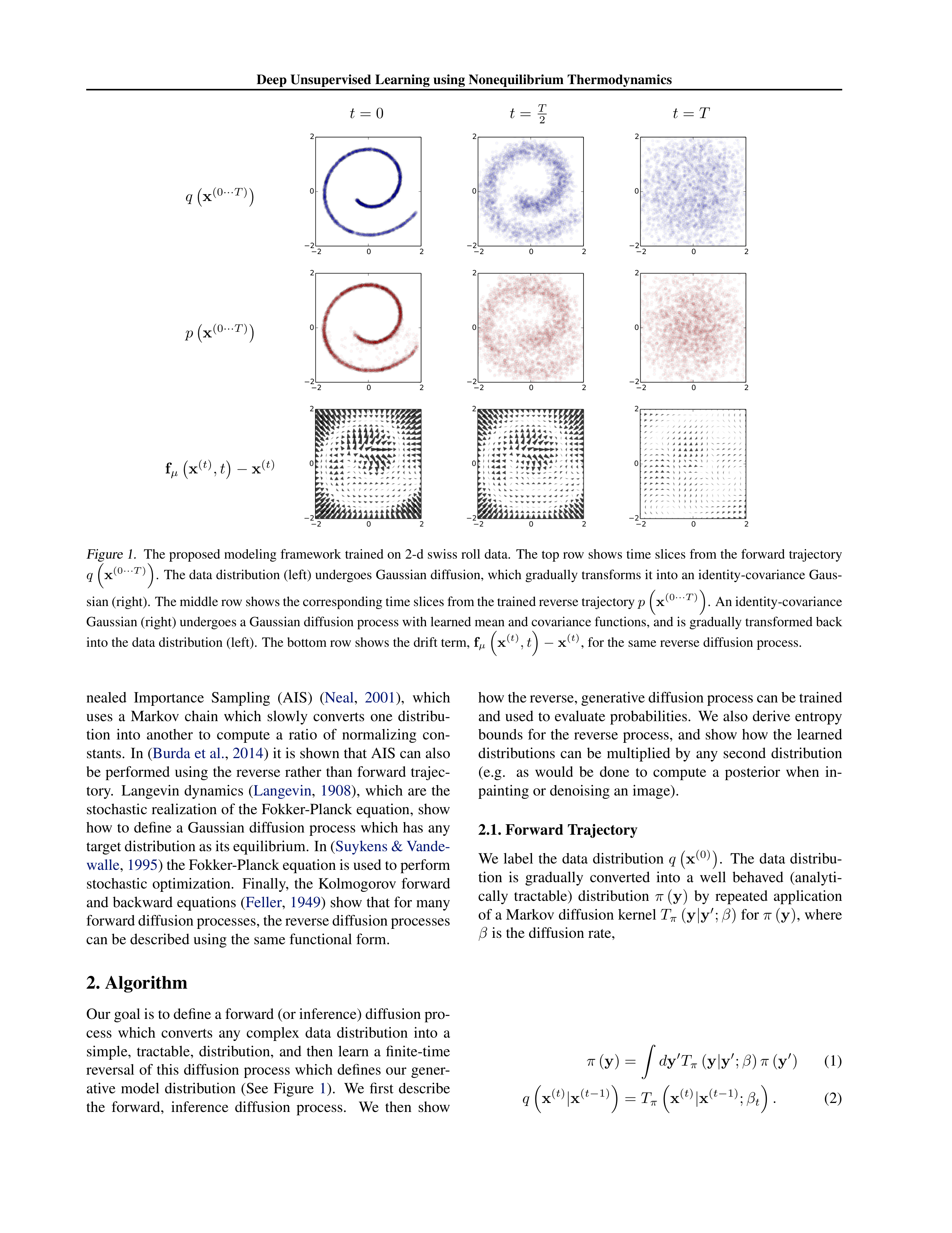
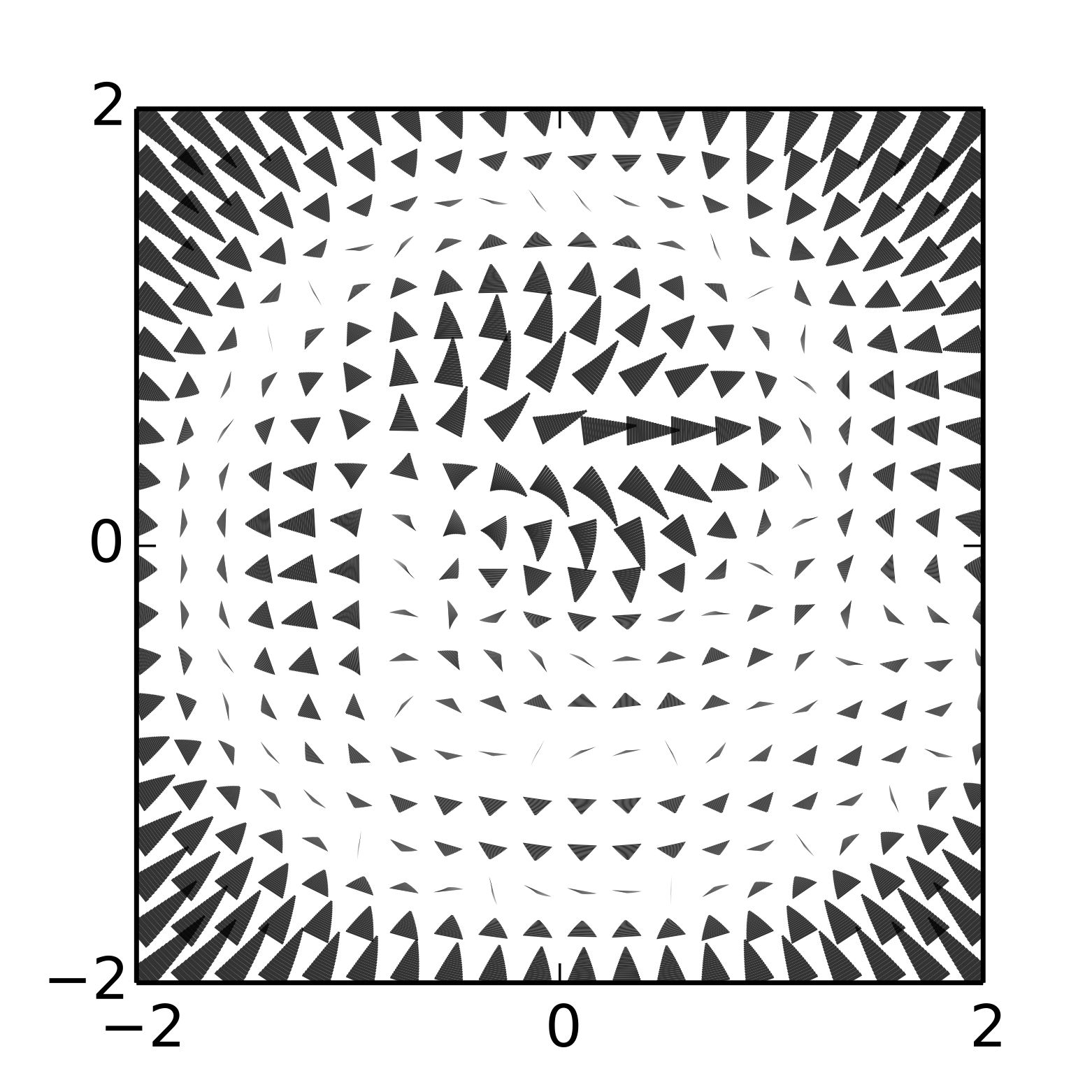
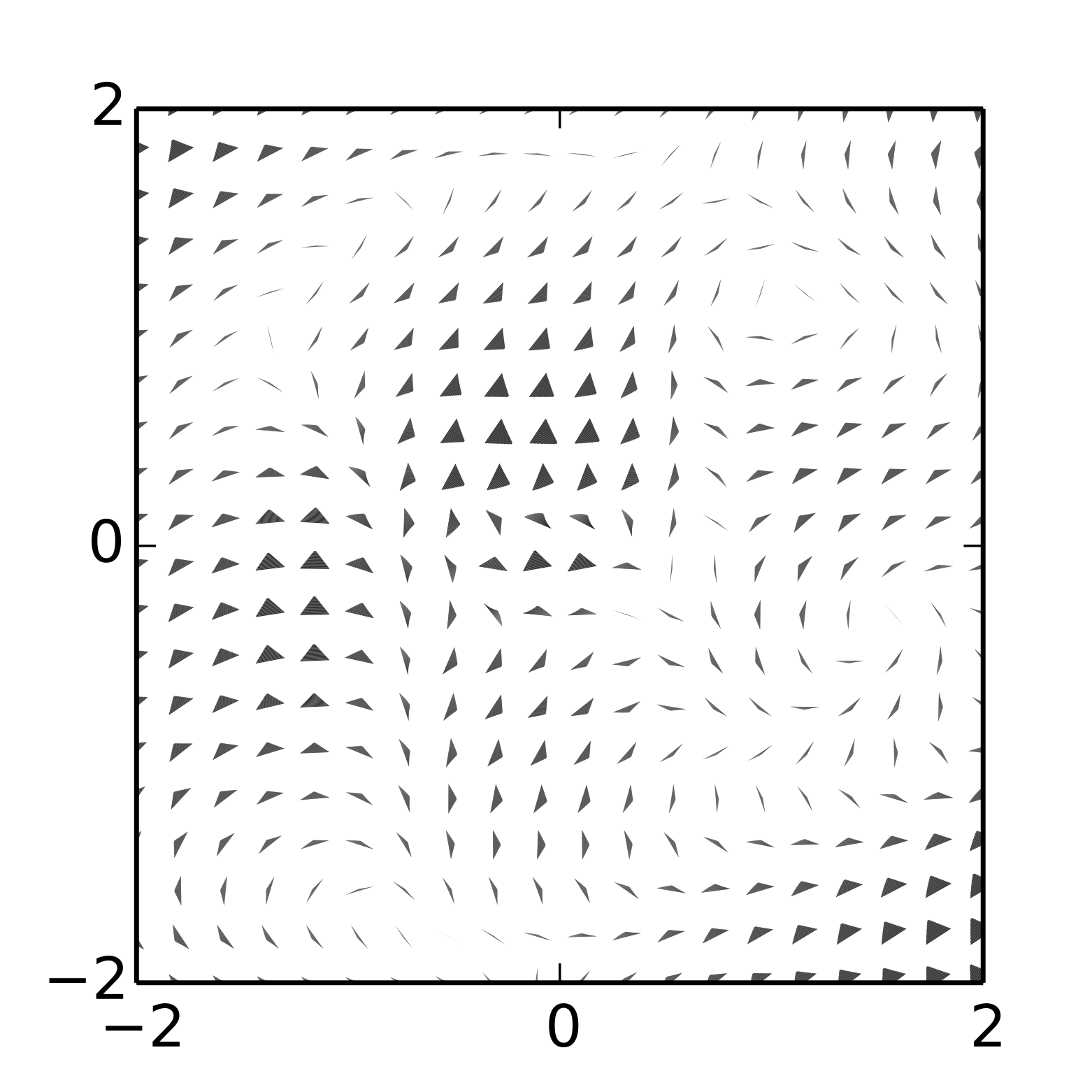
Figure 1.
The proposed modeling framework trained on 2-d swiss roll data.
The top row shows time slices from the forward trajectory
q
x
(0
···
T
)
.
The data distribution (left) undergoes Gaussian diffusion, which gradually transforms it into an identity-covariance Gaus-
sian (right). The middle row shows the corresponding time slices from the trained reverse trajectory
p
x
(0
···
T
)
. An identity-covariance
Gaussian (right) undergoes a Gaussian diffusion process with learned mean and covariance functions, and is gradually transformed back
into the data distribution (left).
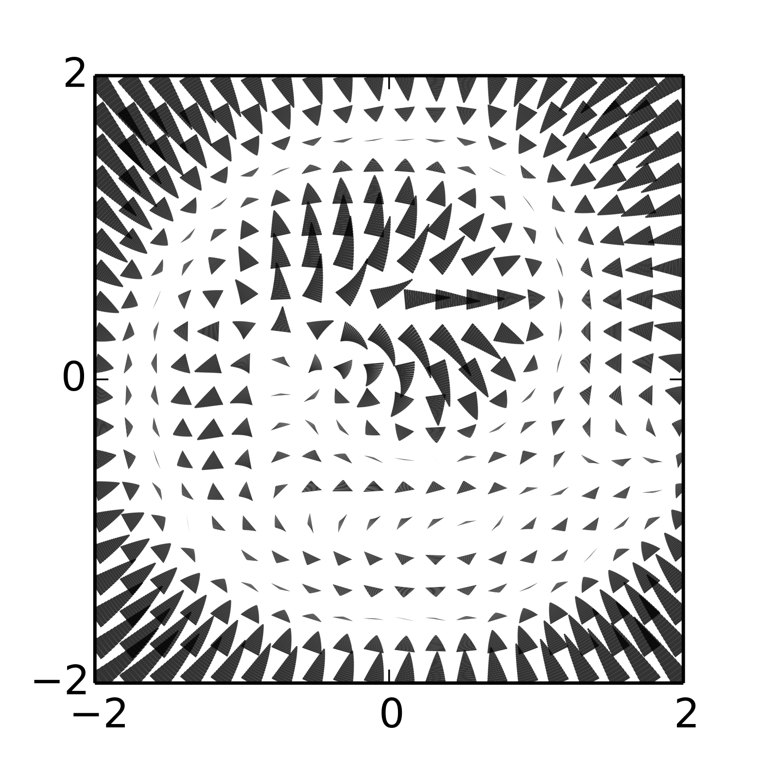
The bottom row shows the drift term,
f
µ
x
(
t
)
, t
−
x
(
t
)
, for the same reverse diffusion process.
nealed
Importance
Sampling
(AIS)
(
Neal
,
2001
),
which
uses
a
Markov
chain
which
slowly
converts
one
distribu-
tion
into
another
to
compute
a
ratio
of
normalizing
con-
stants.
In (
Burda et al.
,
2014
) it is shown that AIS can also
be performed using the reverse rather than forward trajec-
tory.
Langevin
dynamics
(
Langevin
,
1908
),
which
are
the
stochastic realization of the Fokker-Planck equation, show
how to define a Gaussian diffusion process which has any
target distribution as its equilibrium. In (
Suykens & Vande-
walle
,
1995
) the Fokker-Planck equation is used to perform
stochastic
optimization.
Finally,
the
Kolmogorov
forward
and backward equations (
Feller
,
1949
) show that for many
forward diffusion processes, the reverse diffusion processes
can be described using the same functional form.
2. Algorithm
Our goal is to define a forward (or inference) diffusion pro-
cess
which
converts
any
complex
data
distribution
into
a
simple,
tractable,
distribution,
and
then
learn
a
finite-time
reversal of this diffusion process which defines our gener-
ative
model
distribution
(See
Figure
1
).
We
first
describe
the
forward,
inference
diffusion
process.
We
then
show
how the reverse, generative diffusion process can be trained
and used to evaluate probabilities.
We also derive entropy
bounds
for
the
reverse
process,
and
show
how
the
learned
distributions
can
be
multiplied
by
any
second
distribution
(e.g.
as
would
be
done
to
compute
a
posterior
when
in-
painting or denoising an image).
2.1. Forward Trajectory
We
label
the
data
distribution
q
x
(0)
.
The
data
distribu-
tion
is
gradually
converted
into
a
well
behaved
(analyti-
cally
tractable)
distribution
π
(
y
)
by
repeated
application
of a Markov diffusion kernel
T
π
(
y
|
y
′
;
β
)
for
π
(
y
)
, where
β
is the diffusion rate,
π
(
y
) =
Z
d
y
′
T
π
(
y
|
y
′
;
β
)
π
(
y
′
)
(1)
q
x
(
t
)
|
x
(
t
−
1)
=
T
π
x
(
t
)
|
x
(
t
−
1)
;
β
t
.
(2)



Deep Unsupervised Learning using Nonequilibrium Thermodynamics
t
= 0
t
=
T
2
t
=
T
p
x
(0
···
T
)
0
5
10
15
Bin
0
5
10
15
20
Sample
0
5
10
15
Bin
0
5
10
15
20
Sample
0
5
10
15
Bin
0
5
10
15
20
Sample
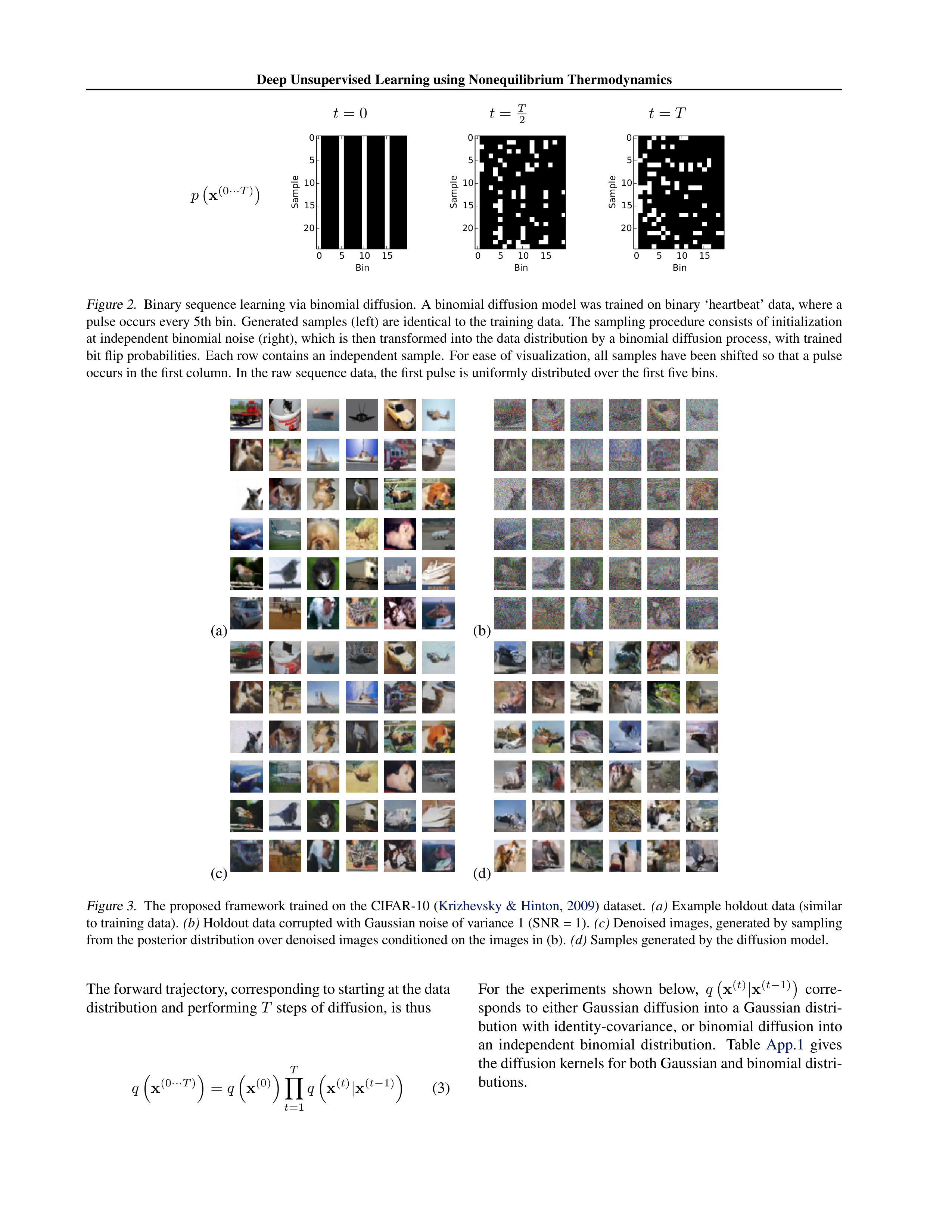
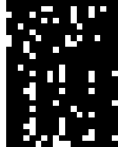
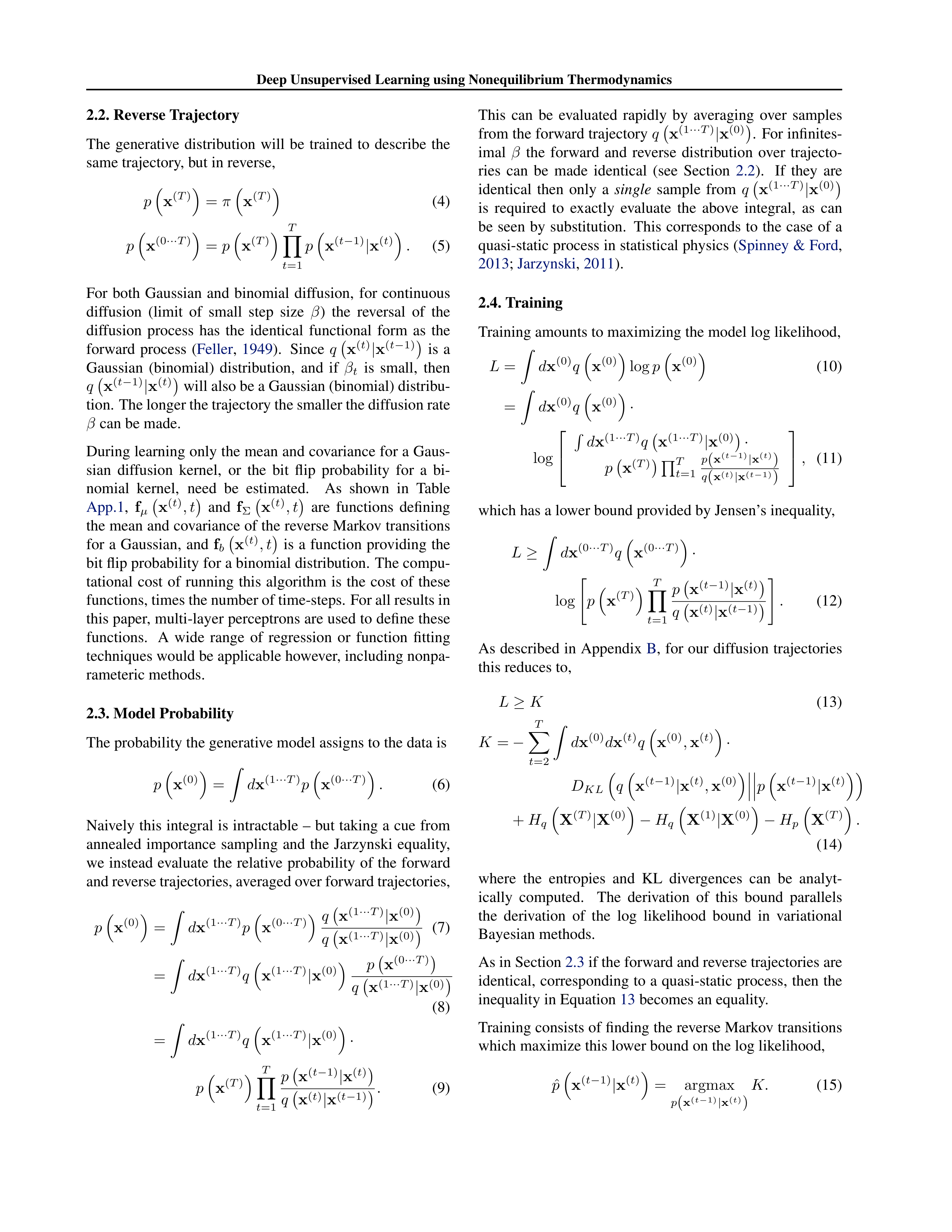
Figure 2.
Binary sequence learning via binomial diffusion.
A binomial diffusion model was trained on binary ‘heartbeat’ data, where a
pulse occurs every 5th bin.
Generated samples (left) are identical to the training data.
The sampling procedure consists of initialization
at independent binomial noise (right), which is then transformed into the data distribution by a binomial diffusion process, with trained
bit flip probabilities.
Each row contains an independent sample.
For ease of visualization, all samples have been shifted so that a pulse
occurs in the first column.
In the raw sequence data, the first pulse is uniformly distributed over the first five bins.
(a)
(b)
(c)
(d)
Figure 3.
The proposed framework trained on the CIFAR-10 (
Krizhevsky & Hinton
,
2009
) dataset.
(a)
Example holdout data (similar
to training data).
(b)
Holdout data corrupted with Gaussian noise of variance 1 (SNR = 1).
(c)
Denoised images, generated by sampling
from the posterior distribution over denoised images conditioned on the images in (b).
(d)
Samples generated by the diffusion model.
The forward trajectory, corresponding to starting at the data
distribution and performing
T
steps of diffusion, is thus
q
x
(0
···
T
)
=
q
x
(0)
T
Y
t
=1
q
x
(
t
)
|
x
(
t
−
1)
(3)
For
the
experiments
shown
below,
q
x
(
t
)
|
x
(
t
−
1)
corre-
sponds to either Gaussian diffusion into a Gaussian distri-
bution with identity-covariance, or binomial diffusion into
an
independent
binomial
distribution.
Table
App.1
gives
the diffusion kernels for both Gaussian and binomial distri-
butions.
Deep Unsupervised Learning using Nonequilibrium Thermodynamics
2.2. Reverse Trajectory
The
generative
distribution
will
be
trained
to
describe
the
same trajectory, but in reverse,
p
x
(
T
)
=
π
x
(
T
)
(4)
p
x
(0
···
T
)
=
p
x
(
T
)
T
Y
t
=1
p
x
(
t
−
1)
|
x
(
t
)
.
(5)
For
both
Gaussian
and
binomial
diffusion,
for
continuous
diffusion
(limit
of
small
step
size
β
)
the
reversal
of
the
diffusion
process
has
the
identical
functional
form
as
the
forward
process
(
Feller
,
1949
).
Since
q
x
(
t
)
|
x
(
t
−
1)
is
a
Gaussian
(binomial)
distribution,
and
if
β
t
is
small,
then
q
x
(
t
−
1)
|
x
(
t
)
will also be a Gaussian (binomial) distribu-
tion. The longer the trajectory the smaller the diffusion rate
β
can be made.
During learning only the mean and covariance for a Gaus-
sian
diffusion
kernel,
or
the
bit
flip
probability
for
a
bi-
nomial
kernel,
need
be
estimated.
As
shown
in
Table
App.1
,
f
µ
x
(
t
)
, t
and
f
Σ
x
(
t
)
, t
are
functions
defining
the mean and covariance of the reverse Markov transitions
for
a
Gaussian,
and
f
b
x
(
t
)
, t
is
a
function
providing
the
bit flip probability for a binomial distribution.
The compu-
tational
cost
of
running
this
algorithm
is
the
cost
of
these
functions, times the number of time-steps.
For all results in
this paper, multi-layer perceptrons are used to define these
functions.
A
wide
range
of
regression
or
function
fitting
techniques would be applicable however, including nonpa-
rameteric methods.
2.3. Model Probability
The probability the generative model assigns to the data is
p
x
(0)
=
Z
d
x
(1
···
T
)
p
x
(0
···
T
)
.
(6)
Naively this integral is intractable – but taking a cue from
annealed
importance
sampling
and
the
Jarzynski
equality,
we
instead
evaluate
the
relative
probability
of
the
forward
and reverse trajectories, averaged over forward trajectories,
p
x
(0)
=
Z
d
x
(1
···
T
)
p
x
(0
···
T
)
q
x
(1
···
T
)
|
x
(0)
q
x
(1
···
T
)
|
x
(0)
(7)
=
Z
d
x
(1
···
T
)
q
x
(1
···
T
)
|
x
(0)
p
x
(0
···
T
)
q
x
(1
···
T
)
|
x
(0)
(8)
=
Z
d
x
(1
···
T
)
q
x
(1
···
T
)
|
x
(0)
·
p
x
(
T
)
T
Y
t
=1
p
x
(
t
−
1)
|
x
(
t
)
q
x
(
t
)
|
x
(
t
−
1)
.
(9)
This
can
be
evaluated
rapidly
by
averaging
over
samples
from the forward trajectory
q
x
(1
···
T
)
|
x
(0)
.
For infinites-
imal
β
the
forward
and
reverse
distribution
over
trajecto-
ries
can
be
made
identical
(see
Section
2.2
).
If
they
are
identical
then
only
a
single
sample
from
q
x
(1
···
T
)
|
x
(0)
is
required
to
exactly
evaluate
the
above
integral,
as
can
be
seen
by
substitution.
This
corresponds
to
the
case
of
a
quasi-static process in statistical physics (
Spinney & Ford
,
2013
;
Jarzynski
,
2011
).
2.4. Training
Training amounts to maximizing the model log likelihood,
L
=
Z
d
x
(0)
q
x
(0)
log
p
x
(0)
(10)
=
Z
d
x
(0)
q
x
(0)
·
log
R
d
x
(1
···
T
)
q
x
(1
···
T
)
|
x
(0)
·
p
x
(
T
)
Q
T
t
=1
p
(
x
(
t
−
1)
|
x
(
t
)
)
q
(
x
(
t
)
|
x
(
t
−
1)
)
,
(11)
which has a lower bound provided by Jensen’s inequality,
L
≥
Z
d
x
(0
···
T
)
q
x
(0
···
T
)
·
log
"
p
x
(
T
)
T
Y
t
=1
p
x
(
t
−
1)
|
x
(
t
)
q
x
(
t
)
|
x
(
t
−
1)
#
.
(12)
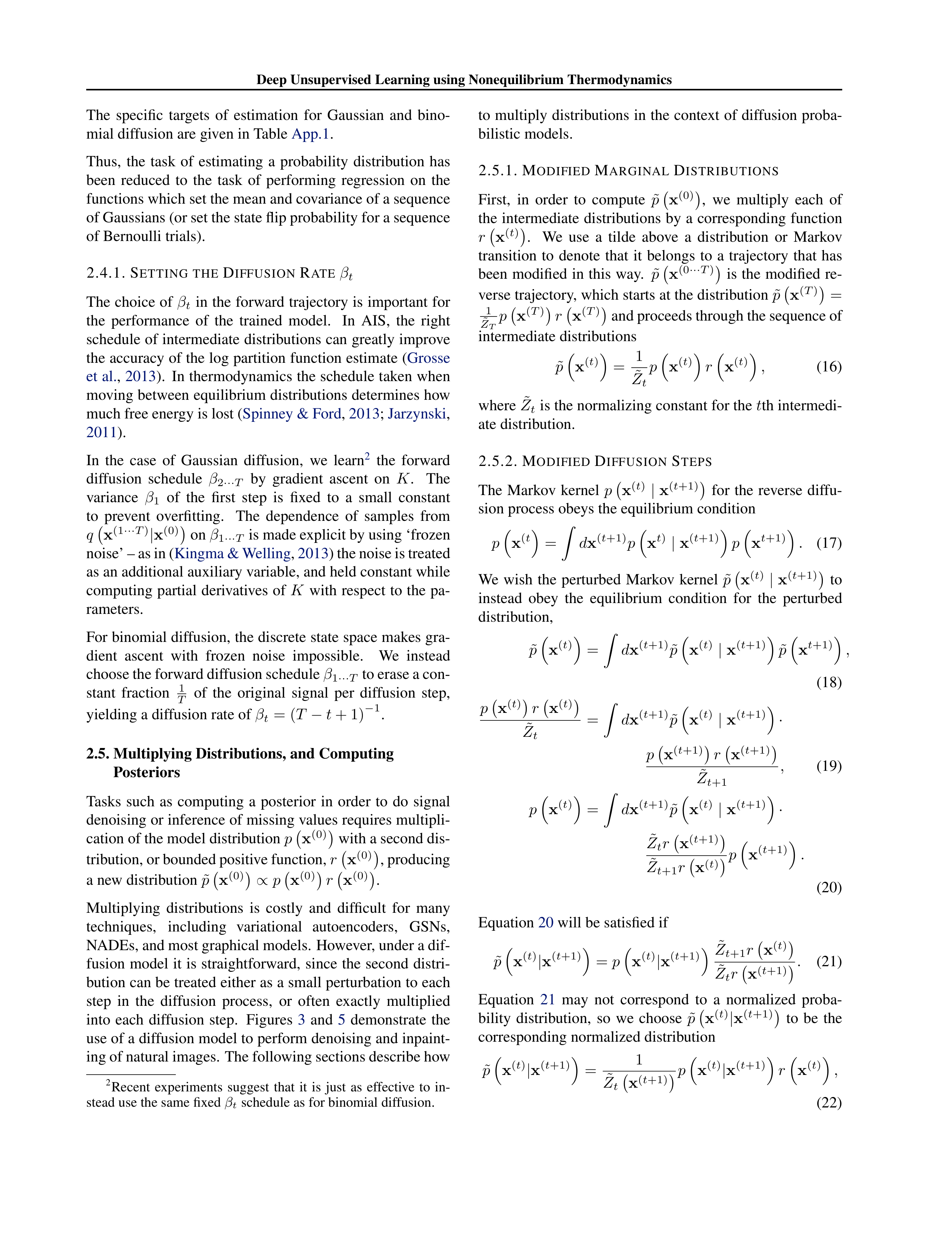
As described in Appendix
B
, for our diffusion trajectories
this reduces to,
L
≥
K
(13)
K
=
−
T
X
t
=2
Z
d
x
(0)
d
x
(
t
)
q
x
(0)
,
x
(
t
)
·
D
KL
q
x
(
t
−
1)
|
x
(
t
)
,
x
(0)
p
x
(
t
−
1)
|
x
(
t
)
+
H
q
X
(
T
)
|
X
(0)
−
H
q
X
(1)
|
X
(0)
−
H
p
X
(
T
)
.
(14)
where
the
entropies
and
KL
divergences
can
be
analyt-
ically
computed.
The
derivation
of
this
bound
parallels
the
derivation
of
the
log
likelihood
bound
in
variational
Bayesian methods.
As in Section
2.3
if the forward and reverse trajectories are
identical,
corresponding to a quasi-static process,
then the
inequality in Equation
13
becomes an equality.
Training consists of finding the reverse Markov transitions
which maximize this lower bound on the log likelihood,
ˆ
p
x
(
t
−
1)
|
x
(
t
)
=
argmax
p
(
x
(
t
−
1)
|
x
(
t
)
)
K.
(15)
Deep Unsupervised Learning using Nonequilibrium Thermodynamics
The
specific
targets
of
estimation
for
Gaussian
and
bino-
mial diffusion are given in Table
App.1
.
Thus,
the
task
of
estimating
a
probability
distribution
has
been
reduced
to
the
task
of
performing
regression
on
the
functions which set the mean and covariance of a sequence
of Gaussians (or set the state flip probability for a sequence
of Bernoulli trials).
2.4.1. S
ETTING
THE
D
IFFUSION
R
ATE
β
t
The choice of
β
t
in the forward trajectory is important for
the
performance
of
the
trained
model.
In
AIS,
the
right
schedule of intermediate distributions can greatly improve
the accuracy of the log partition function estimate (
Grosse
et al.
,
2013
).
In thermodynamics the schedule taken when
moving between equilibrium distributions determines how
much free energy is lost (
Spinney & Ford
,
2013
;
Jarzynski
,
2011
).
In
the
case
of
Gaussian
diffusion,
we
learn
2
the
forward
diffusion
schedule
β
2
···
T
by
gradient
ascent
on
K
.
The
variance
β
1
of
the
first
step
is
fixed
to
a
small
constant
to
prevent
overfitting.
The
dependence
of
samples
from
q
x
(1
···
T
)
|
x
(0)
on
β
1
···
T
is made explicit by using ‘frozen
noise’ – as in (
Kingma & Welling
,
2013
) the noise is treated
as an additional auxiliary variable, and held constant while
computing
partial
derivatives
of
K
with
respect
to
the
pa-
rameters.
For binomial diffusion, the discrete state space makes gra-
dient
ascent
with
frozen
noise
impossible.
We
instead
choose the forward diffusion schedule
β
1
···
T
to erase a con-
stant
fraction
1
T
of
the
original
signal
per
diffusion
step,
yielding a diffusion rate of
β
t
= (
T
−
t
+ 1)
−
1
.
2.5. Multiplying Distributions, and Computing
Posteriors
Tasks
such
as
computing
a
posterior
in
order
to
do
signal
denoising or inference of missing values requires multipli-
cation of the model distribution
p
x
(0)
with a second dis-
tribution, or bounded positive function,
r
x
(0)
, producing
a new distribution
˜
p
x
(0)
∝
p
x
(0)
r
x
(0)
.
Multiplying
distributions
is
costly
and
difficult
for
many
techniques,
including
variational
autoencoders,
GSNs,
NADEs, and most graphical models.
However, under a dif-
fusion
model it
is
straightforward,
since
the
second
distri-
bution can be treated either as a small perturbation to each
step
in
the
diffusion
process,
or
often
exactly
multiplied
into
each
diffusion
step.
Figures
3
and
5
demonstrate
the
use of a diffusion model to perform denoising and inpaint-
ing of natural images.
The following sections describe how
2
Recent
experiments
suggest
that
it
is
just
as
effective
to
in-
stead use the same fixed
β
t
schedule as for binomial diffusion.
to multiply distributions in the context of diffusion proba-
bilistic models.
2.5.1. M
ODIFIED
M
ARGINAL
D
ISTRIBUTIONS
First,
in
order
to
compute
˜
p
x
(0)
,
we
multiply
each
of
the intermediate distributions by a corresponding function
r
x
(
t
)
.
We
use
a
tilde
above
a
distribution
or
Markov
transition
to
denote
that
it
belongs
to
a
trajectory
that
has
been
modified
in this
way.
˜
p
x
(0
···
T
)
is the
modified re-
verse trajectory, which starts at the distribution
˜
p
x
(
T
)
=
1
˜
Z
T
p
x
(
T
)
r
x
(
T
)
and proceeds through the sequence of
intermediate distributions
˜
p
x
(
t
)
=
1
˜
Z
t
p
x
(
t
)
r
x
(
t
)
,
(16)
where
˜
Z
t
is the normalizing constant for the
t
th intermedi-
ate distribution.
2.5.2. M
ODIFIED
D
IFFUSION
S
TEPS
The
Markov
kernel
p
x
(
t
)
|
x
(
t
+1)
for
the
reverse
diffu-
sion process obeys the equilibrium condition
p
x
(
t
=
Z
d
x
(
t
+1)
p
x
t
)
|
x
(
t
+1)
p
x
t
+1)
.
(17)
We
wish
the
perturbed
Markov
kernel
˜
p
x
(
t
)
|
x
(
t
+1)
to
instead
obey
the
equilibrium
condition
for
the
perturbed
distribution,
˜
p
x
(
t
)
=
Z
d
x
(
t
+1)
˜
p
x
(
t
)
|
x
(
t
+1)
˜
p
x
t
+1)
,
(18)
p
x
(
t
)
r
x
(
t
)
˜
Z
t
=
Z
d
x
(
t
+1)
˜
p
x
(
t
)
|
x
(
t
+1)
·
p
x
(
t
+1)
r
x
(
t
+1)
˜
Z
t
+1
,
(19)
p
x
(
t
)
=
Z
d
x
(
t
+1)
˜
p
x
(
t
)
|
x
(
t
+1)
·
˜
Z
t
r
x
(
t
+1)
˜
Z
t
+1
r
x
(
t
)
p
x
(
t
+1)
.
(20)
Equation
20
will be satisfied if
˜
p
x
(
t
)
|
x
(
t
+1)
=
p
x
(
t
)
|
x
(
t
+1)
˜
Z
t
+1
r
x
(
t
)
˜
Z
t
r
x
(
t
+1)
.
(21)
Equation
21
may
not
correspond
to
a
normalized
proba-
bility
distribution,
so
we
choose
˜
p
x
(
t
)
|
x
(
t
+1)
to
be
the
corresponding normalized distribution
˜
p
x
(
t
)
|
x
(
t
+1)
=
1
˜
Z
t
x
(
t
+1)
p
x
(
t
)
|
x
(
t
+1)
r
x
(
t
)
,
(22)
Deep Unsupervised Learning using Nonequilibrium Thermodynamics
(a)
0
50
100
150
200
250
0
50
100
150
200
250
(b)
0
50
100
150
200
250
0
50
100
150
200
250
(c)
0
50
100
150
200
250
0
50
100
150
200
250
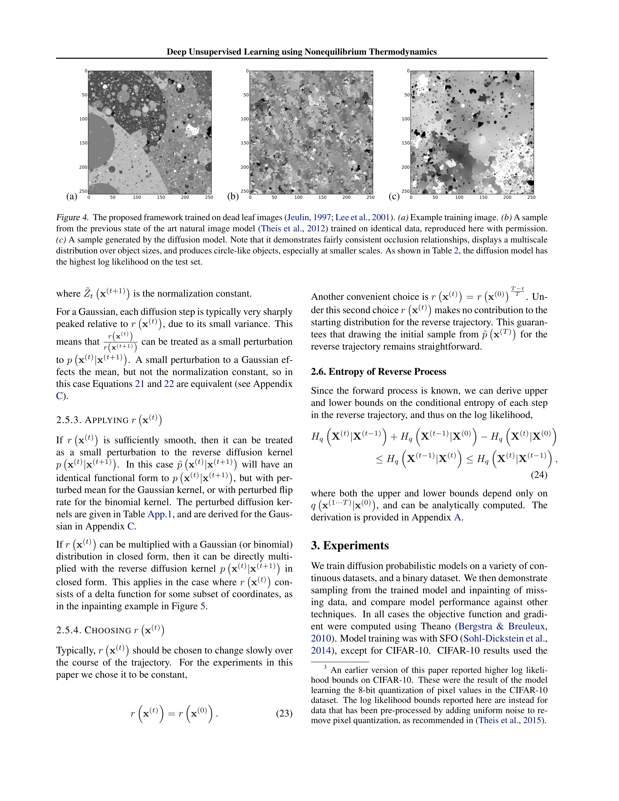
Figure 4.
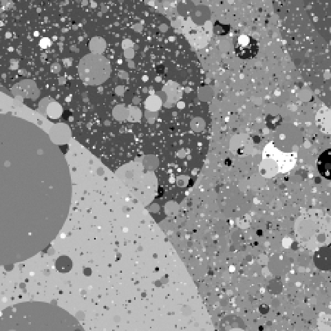
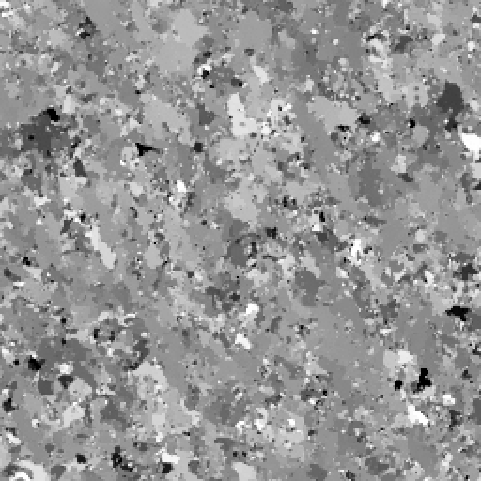
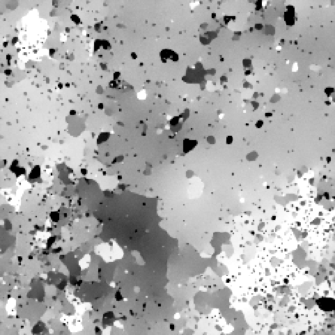
The proposed framework trained on dead leaf images (
Jeulin
,
1997
;
Lee et al.
,
2001
).
(a)
Example training image.
(b)
A sample
from
the
previous
state
of
the
art
natural
image
model
(
Theis
et
al.
,
2012
)
trained
on
identical
data,
reproduced
here
with
permission.
(c)
A sample generated by the diffusion model.
Note that it demonstrates fairly consistent occlusion relationships, displays a multiscale
distribution over object sizes, and produces circle-like objects, especially at smaller scales.
As shown in Table
2
, the diffusion model has
the highest log likelihood on the test set.
where
˜
Z
t
x
(
t
+1)
is the normalization constant.
For a Gaussian, each diffusion step is typically very sharply
peaked relative to
r
x
(
t
)
,
due to its small variance.
This
means that
r
(
x
(
t
)
)
r
(
x
(
t
+1)
)
can be treated as a small perturbation
to
p
x
(
t
)
|
x
(
t
+1)
.
A
small
perturbation
to
a
Gaussian
ef-
fects
the
mean,
but
not
the
normalization
constant,
so
in
this case Equations
21
and
22
are equivalent (see Appendix
C
).
2.5.3. A
PPLYING
r
x
(
t
)
If
r
x
(
t
)
is
sufficiently
smooth,
then
it
can
be
treated
as
a
small
perturbation
to
the
reverse
diffusion
kernel
p
x
(
t
)
|
x
(
t
+1)
.
In
this
case
˜
p
x
(
t
)
|
x
(
t
+1)
will
have
an
identical
functional
form
to
p
x
(
t
)
|
x
(
t
+1)
,
but
with
per-
turbed mean for the Gaussian kernel, or with perturbed flip
rate
for
the
binomial
kernel.
The
perturbed
diffusion
ker-
nels are given in Table
App.1
, and are derived for the Gaus-
sian in Appendix
C
.
If
r
x
(
t
)
can be multiplied with a Gaussian (or binomial)
distribution
in
closed
form,
then
it
can
be
directly
multi-
plied
with
the
reverse
diffusion
kernel
p
x
(
t
)
|
x
(
t
+1)
in
closed
form.
This
applies
in
the
case
where
r
x
(
t
)
con-
sists of a delta function for some subset of coordinates, as
in the inpainting example in Figure
5
.
2.5.4. C
HOOSING
r
x
(
t
)
Typically,
r
x
(
t
)
should be chosen to change slowly over
the
course
of
the
trajectory.
For
the
experiments
in
this
paper we chose it to be constant,
r
x
(
t
)
=
r
x
(0)
.
(23)
Another convenient choice is
r
x
(
t
)
=
r
x
(0)
T
−
t
T
.
Un-
der this second choice
r
x
(
t
)
makes no contribution to the
starting distribution for the reverse trajectory.
This guaran-
tees
that
drawing
the
initial
sample
from
˜
p
x
(
T
)
for
the
reverse trajectory remains straightforward.
2.6. Entropy of Reverse Process
Since
the
forward
process
is
known,
we
can
derive
upper
and
lower
bounds
on
the
conditional
entropy
of
each
step
in the reverse trajectory, and thus on the log likelihood,
H
q
X
(
t
)
|
X
(
t
−
1)
+
H
q
X
(
t
−
1)
|
X
(0)
−
H
q
X
(
t
)
|
X
(0)
≤
H
q
X
(
t
−
1)
|
X
(
t
)
≤
H
q
X
(
t
)
|
X
(
t
−
1)
,
(24)
where
both
the
upper
and
lower
bounds
depend
only
on
q
x
(1
···
T
)
|
x
(0)
,
and
can
be
analytically
computed.
The
derivation is provided in Appendix
A
.
3. Experiments
We train diffusion probabilistic models on a variety of con-
tinuous datasets, and a binary dataset. We then demonstrate
sampling
from
the
trained
model
and
inpainting
of
miss-
ing
data,
and
compare
model
performance
against
other
techniques.
In
all
cases
the
objective
function
and
gradi-
ent
were
computed
using
Theano
(
Bergstra
&
Breuleux
,
2010
). Model training was with SFO (
Sohl-Dickstein et al.
,
2014
),
except
for
CIFAR-10.
CIFAR-10
results
used
the
3
An
earlier
version
of
this
paper
reported
higher
log
likeli-
hood
bounds
on
CIFAR-10.
These
were
the
result
of
the
model
learning
the
8-bit
quantization
of
pixel
values
in
the
CIFAR-10
dataset.
The
log
likelihood
bounds
reported
here
are
instead
for
data
that
has
been
pre-processed
by
adding
uniform
noise
to
re-
move pixel quantization, as recommended in (
Theis et al.
,
2015
).
Deep Unsupervised Learning using Nonequilibrium Thermodynamics
(a)
0
50
100
150
200
250
300
0
50
100
150
200
250
300
(b)
0
50
100
150
200
250
300
0
50
100
150
200
250
300
(c)
0
50
100
150
200
250
300
0
50
100
150
200
250
300
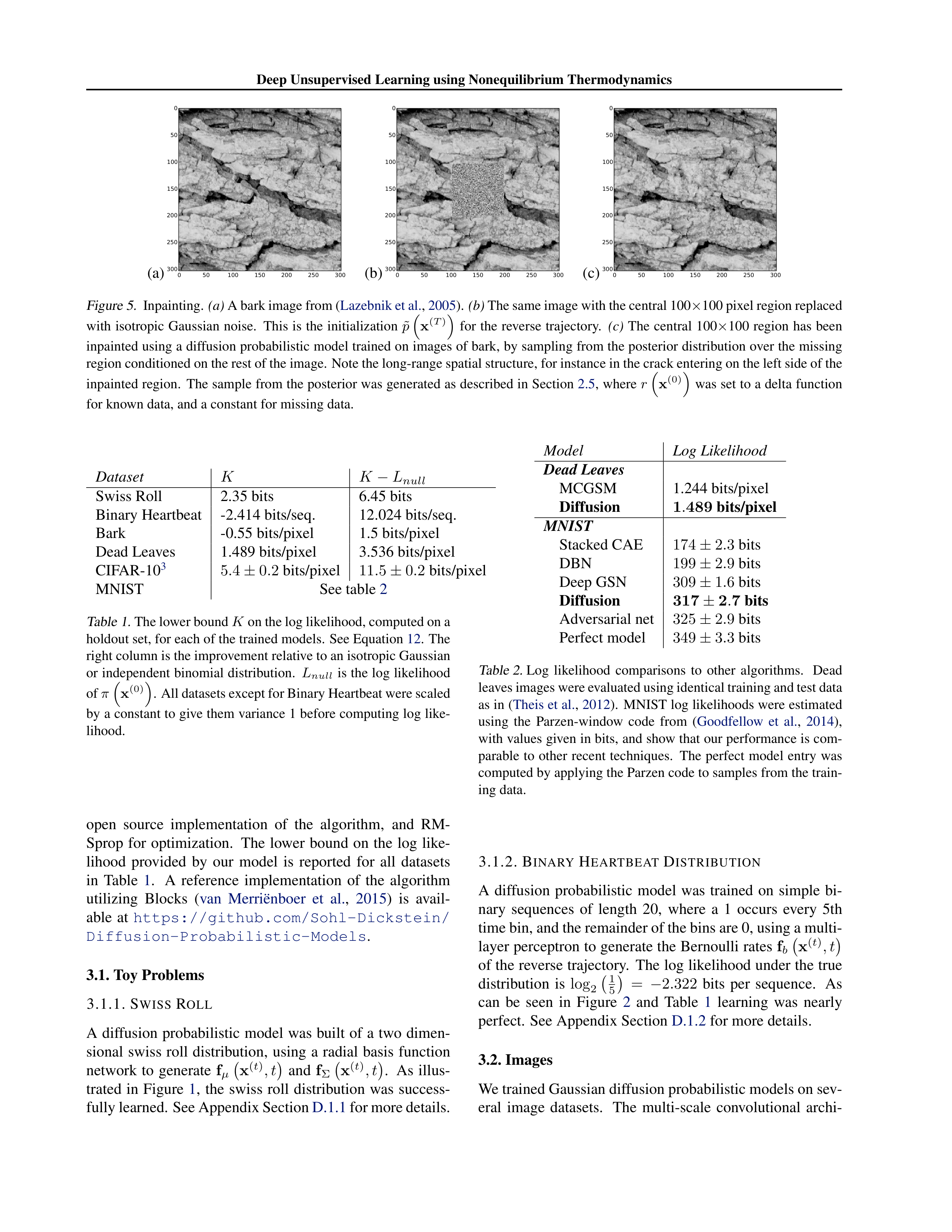
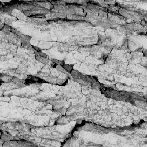
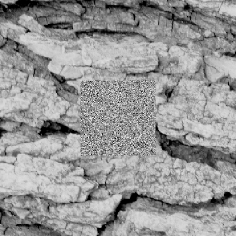
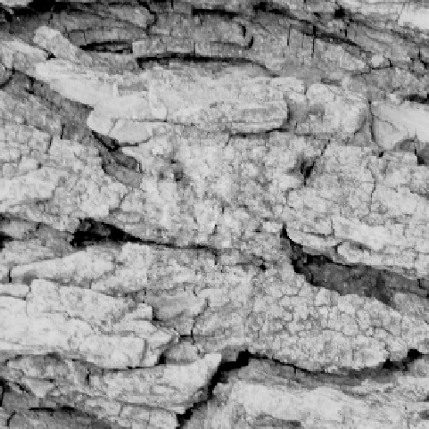
Figure 5.
Inpainting.
(a)
A bark image from (
Lazebnik et al.
,
2005
).
(b)
The same image with the central 100
×
100 pixel region replaced
with
isotropic
Gaussian
noise.
This
is
the
initialization
˜
p
x
(
T
)
for
the
reverse
trajectory.
(c)
The
central
100
×
100
region
has
been
inpainted using a diffusion probabilistic model trained on images of bark, by sampling from the posterior distribution over the missing
region conditioned on the rest of the image.
Note the long-range spatial structure, for instance in the crack entering on the left side of the
inpainted region.
The sample from the posterior was generated as described in Section
2.5
, where
r
x
(0)
was set to a delta function
for known data, and a constant for missing data.
Dataset
K
K
−
L
null
Swiss Roll
2.35 bits
6.45 bits
Binary Heartbeat
-2.414 bits/seq.
12.024 bits/seq.
Bark
-0.55 bits/pixel
1.5 bits/pixel
Dead Leaves
1.489 bits/pixel
3.536 bits/pixel
CIFAR-10
3
5
.
4
±
0
.
2
bits/pixel
11
.
5
±
0
.
2
bits/pixel
MNIST
See table
2
Table 1.
The lower bound
K
on the log likelihood, computed on a
holdout set, for each of the trained models.
See Equation
12
.
The
right column is the improvement relative to an isotropic Gaussian
or independent binomial distribution.
L
null
is the log likelihood
of
π
x
(0)
. All datasets except for Binary Heartbeat were scaled
by a constant to give them variance 1 before computing log like-
lihood.
open
source
implementation
of
the
algorithm,
and
RM-
Sprop
for
optimization.
The
lower
bound
on
the
log
like-
lihood
provided
by
our
model
is
reported
for
all
datasets
in
Table
1
.
A
reference
implementation
of
the
algorithm
utilizing
Blocks
(
van
Merri¨enboer
et
al.
,
2015
)
is
avail-
able
at
https://github.com/Sohl-Dickstein/
Diffusion-Probabilistic-Models
.
3.1. Toy Problems
3.1.1. S
WISS
R
OLL
A
diffusion
probabilistic
model
was
built
of
a
two
dimen-
sional
swiss
roll
distribution,
using
a
radial
basis
function
network
to
generate
f
µ
x
(
t
)
, t
and
f
Σ
x
(
t
)
, t
.
As
illus-
trated
in
Figure
1
,
the
swiss
roll
distribution
was
success-
fully learned. See Appendix Section
D.1.1
for more details.
Model
Log Likelihood
Dead Leaves
MCGSM
1.244 bits/pixel
Diffusion
1
.
489
bits/pixel
MNIST
Stacked CAE
174
±
2
.
3
bits
DBN
199
±
2
.
9
bits
Deep GSN
309
±
1
.
6
bits
Diffusion
317
±
2
.
7
bits
Adversarial net
325
±
2
.
9
bits
Perfect model
349
±
3
.
3
bits
Table 2.
Log
likelihood
comparisons
to
other
algorithms.
Dead
leaves images were evaluated using identical training and test data
as in (
Theis et al.
,
2012
).
MNIST log likelihoods were estimated
using
the
Parzen-window
code
from
(
Goodfellow
et
al.
,
2014
),
with values given in bits, and show that our performance is com-
parable
to
other
recent
techniques.
The
perfect
model
entry
was
computed by applying the Parzen code to samples from the train-
ing data.
3.1.2. B
INARY
H
EARTBEAT
D
ISTRIBUTION
A
diffusion
probabilistic
model
was
trained
on
simple
bi-
nary
sequences
of
length
20,
where
a
1
occurs
every
5th
time bin, and the remainder of the bins are 0, using a multi-
layer perceptron to generate the Bernoulli rates
f
b
x
(
t
)
, t
of the reverse trajectory.
The log likelihood under the true
distribution
is
log
2
1
5
=
−
2
.
322
bits
per
sequence.
As
can
be
seen
in
Figure
2
and
Table
1
learning
was
nearly
perfect.
See Appendix Section
D.1.2
for more details.
3.2. Images
We trained Gaussian diffusion probabilistic models on sev-
eral
image
datasets.
The
multi-scale
convolutional
archi-
Deep Unsupervised Learning using Nonequilibrium Thermodynamics
tecture
shared
by
these
experiments
is
described
in
Ap-
pendix Section
D.2.1
, and illustrated in Figure
D.1
.
3.2.1. D
ATASETS
MNIST
In
order
to
allow
a
direct
comparison
against
previous
work
on
a
simple
dataset,
we
trained
on
MNIST
digits (
LeCun & Cortes
,
1998
).
Log likelihoods relative to
(
Bengio
et
al.
,
2012
;
Bengio
&
Thibodeau-Laufer
,
2013
;
Goodfellow
et
al.
,
2014
)
are
given
in
Table
2
.
Samples
from
the
MNIST
model
are
given
in
Appendix
Figure
App.1
.
Our training algorithm provides an asymptotically
consistent
lower
bound
on
the
log
likelihood.
However
most
previous
reported
results
on
continuous
MNIST
log
likelihood
rely
on
Parzen-window
based
estimates
com-
puted from model samples.
For this comparison we there-
fore
estimate
MNIST
log
likelihood
using
the
Parzen-
window code released with (
Goodfellow et al.
,
2014
).
CIFAR-10
A
probabilistic
model
was
fit
to
the
training
images for the CIFAR-10 challenge dataset (
Krizhevsky &
Hinton
,
2009
).
Samples
from
the
trained
model
are
pro-
vided in Figure
3
.
Dead Leaf Images
Dead leaf images (
Jeulin
,
1997
;
Lee
et
al.
,
2001
)
consist
of
layered
occluding
circles,
drawn
from a power law distribution over scales. They have an an-
alytically tractable structure, but capture many of the statis-
tical complexities of natural images, and therefore provide
a compelling test case for natural image models.
As illus-
trated
in
Table
2
and
Figure
4
,
we
achieve
state
of
the
art
performance on the dead leaves dataset.
Bark Texture Images
A probabilistic model was trained
on
bark
texture
images
(T01-T04)
from
(
Lazebnik
et
al.
,
2005
). For this dataset we demonstrate that it is straightfor-
ward
to
evaluate
or
generate
from
a
posterior
distribution,
by inpainting a large region of missing data using a sample
from the model posterior in Figure
5
.
4. Conclusion
We have introduced a novel algorithm for modeling proba-
bility distributions that enables exact sampling and evalua-
tion of probabilities and demonstrated its effectiveness on a
variety of toy and real datasets, including challenging natu-
ral image datasets. For each of these tests we used a similar
basic
algorithm,
showing
that
our
method
can
accurately
model
a
wide
variety
of
distributions.
Most
existing
den-
sity
estimation
techniques
must
sacrifice
modeling
power
in
order
to
stay
tractable
and
efficient,
and
sampling
or
evaluation are often extremely expensive.
The core of our
algorithm
consists
of
estimating
the
reversal
of
a
Markov
diffusion chain which maps data to a noise distribution; as
the number of steps is made large, the reversal distribution
of each diffusion step becomes simple and easy to estimate.
The result is an algorithm that can learn a fit to any data dis-
tribution, but which remains tractable to train,
exactly
sam-
ple
from,
and
evaluate,
and
under
which
it
is
straightfor-
ward to manipulate conditional and posterior distributions.
Acknowledgements
We
thank
Lucas
Theis,
Subhaneil
Lahiri,
Ben
Poole,
Diederik
P.
Kingma,
Taco
Cohen,
Philip
Bachman,
and
A¨aron van den Oord for extremely helpful discussion, and
Ian Goodfellow for Parzen-window code.
We thank Khan
Academy
and
the
Office
of
Naval
Research
for
funding
Jascha
Sohl-Dickstein,
and
we
thank
the
Office
of
Naval
Research
and
the
Burroughs-Wellcome,
Sloan,
and
James
S. McDonnell foundations for funding Surya Ganguli.
References
Barron, J. T., Biggin, M. D., Arbelaez, P., Knowles, D. W.,
Keranen, S. V., and Malik, J.
Volumetric Semantic Seg-
mentation
Using
Pyramid
Context
Features.
In
2013
IEEE International Conference on Computer Vision
, pp.
3448–3455. IEEE, December 2013.
ISBN 978-1-4799-
2840-8.
doi:
10.1109/ICCV.2013.428.
Bengio,
Y.
and
Thibodeau-Laufer,
E.
Deep
genera-
tive
stochastic
networks
trainable
by
backprop.
arXiv
preprint arXiv:1306.1091
, 2013.
Bengio,
Y.,
Mesnil,
G.,
Dauphin,
Y.,
and
Rifai,
S.
Bet-
ter
Mixing
via
Deep
Representations.
arXiv
preprint
arXiv:1207.4404
, July 2012.
Bergstra,
J.
and
Breuleux,
O.
Theano:
a
CPU
and
GPU
math
expression
compiler.
Proceedings
of
the
Python
for Scientific Computing Conference (SciPy)
, 2010.
Besag,
J.
Statistical
Analysis
of
Non-Lattice
Data.
The
Statistician, 24(3), 179-195
, 1975.
Bishop, C., Svens´en, M., and Williams, C.
GTM: The gen-
erative topographic mapping.
Neural computation
, 1998.
Bornschein,
J.
and
Bengio,
Y.
Reweighted
Wake-Sleep.
International
Conference
on
Learning
Representations
,
June 2015.
Burda,
Y.,
Grosse,
R.
B.,
and
Salakhutdinov,
R.
Accu-
rate and Conservative Estimates of MRF Log-likelihood
using
Reverse
Annealing.
arXiv:1412.8566
,
December
2014.
Dayan, P., Hinton, G. E., Neal, R. M., and Zemel, R. S. The
helmholtz machine.
Neural computation
, 7(5):889–904,
1995.
Deep Unsupervised Learning using Nonequilibrium Thermodynamics
Dinh,
L.,
Krueger,
D.,
and
Bengio,
Y.
NICE:
Non-linear
Independent Components Estimation.
arXiv:1410.8516
,
pp.
11, October 2014.
Feller, W.
On the theory of stochastic processes, with par-
ticular
reference
to
applications.
In
Proceedings
of
the
[First]
Berkeley
Symposium
on
Mathematical
Statistics
and Probability
. The
Regents of the
University of Cali-
fornia, 1949.
Gershman,
S.
J.
and
Blei,
D.
M.
A
tutorial
on
Bayesian
nonparametric
models.
Journal
of
Mathematical
Psy-
chology
, 56(1):1–12, 2012.
Gneiting, T. and Raftery, A. E. Strictly proper scoring rules,
prediction, and estimation.
Journal of the American Sta-
tistical Association
, 102(477):359–378, 2007.
Goodfellow,
I.
J.,
Pouget-Abadie,
J.,
Mirza,
M.,
Xu,
B.,
Warde-Farley,
D.,
Ozair,
S.,
Courville,
A.,
and
Bengio,
Y.
Generative
Adversarial
Nets.
Advances
in
Neural
Information Processing Systems
, 2014.
Gregor, K., Danihelka, I., Mnih, A., Blundell, C., and Wier-
stra, D.
Deep AutoRegressive Networks.
arXiv preprint
arXiv:1310.8499
, October 2013.
Grosse, R. B., Maddison, C. J., and Salakhutdinov, R.
An-
nealing between distributions by averaging moments.
In
Advances in Neural Information Processing Systems
, pp.
2769–2777, 2013.
Hinton,
G.
E.
Training
products
of
experts
by
minimiz-
ing contrastive divergence.
Neural Computation
, 14(8):
1771–1800, 2002.
Hinton,
G. E.
The wake-sleep algorithm for unsupervised
neural networks ).
Science
, 1995.
Hyv¨arinen,
A.
Estimation
of
non-normalized
statistical
models
using
score
matching.
Journal
of
Machine
Learning Research
, 6:695–709, 2005.
Jarzynski,
C.
Equilibrium
free-energy
differences
from
nonequilibrium
measurements:
A
master-equation
ap-
proach.
Physical Review E
, January 1997.
Jarzynski,
C.
Equalities
and
inequalities:
irreversibility
and the second law of thermodynamics at the nanoscale.
Annu. Rev. Condens. Matter Phys.
, 2011.
Jeulin,
D.
Dead
leaves
models:
from
space
tesselation
to
random
functions.
Proc.
of
the
Symposium
on
the
Ad-
vances
in the
Theory
and
Applications
of
Random
Sets
,
1997.
Jordan,
M.
I.,
Ghahramani,
Z.,
Jaakkola,
T.
S.,
and
Saul,
L. K.
An introduction to variational methods for graphi-
cal models.
Machine learning
, 37(2):183–233, 1999.
Kavukcuoglu,
K.,
Ranzato,
M.,
and LeCun,
Y.
Fast infer-
ence in sparse coding algorithms with applications to ob-
ject recognition.
arXiv preprint arXiv:1010.3467
, 2010.
Kingma, D. P. and Welling, M.
Auto-Encoding Variational
Bayes.
International Conference on Learning Represen-
tations
, December 2013.
Krizhevsky, A. and Hinton, G.
Learning multiple layers of
features
from
tiny
images.
Computer
Science
Depart-
ment University of Toronto Tech. Rep.
, 2009.
Langevin,
P.
Sur
la
th´eorie
du
mouvement
brownien.
CR
Acad. Sci. Paris
, 146(530-533), 1908.
Larochelle,
H.
and
Murray,
I.
The
neural
autoregressive
distribution estimator.
Journal of Machine Learning Re-
search
, 2011.
Lazebnik,
S.,
Schmid,
C.,
and
Ponce,
J.
A
sparse
texture
representation using local affine regions.
Pattern Analy-
sis and Machine Intelligence, IEEE Transactions on
, 27
(8):1265–1278, 2005.
LeCun,
Y.
and
Cortes,
C.
The
MNIST
database
of
hand-
written digits.
1998.
Lee, A., Mumford, D., and Huang, J. Occlusion models for
natural
images:
A
statistical
study
of
a
scale-invariant
dead
leaves
model.
International
Journal
of
Computer
Vision
, 2001.
Lyu, S.
Unifying Non-Maximum Likelihood Learning Ob-
jectives
with
Minimum
KL
Contraction.
Advances
in
Neural
Information
Processing
Systems
24
,
pp.
64–72,
2011.
MacKay,
D.
Bayesian
neural
networks
and
density
net-
works.
Nuclear Instruments and Methods in Physics Re-
search
Section
A:
Accelerators,
Spectrometers,
Detec-
tors and Associated Equipment
, 1995.
Murphy,
K.
P.,
Weiss,
Y.,
and
Jordan,
M.
I.
Loopy
be-
lief
propagation
for
approximate
inference:
An
empiri-
cal study.
In
Proceedings of the Fifteenth conference on
Uncertainty in artificial intelligence
, pp. 467–475. Mor-
gan Kaufmann Publishers Inc., 1999.
Neal,
R.
Annealed
importance
sampling.
Statistics
and
Computing
, January 2001.
Ozair,
S.
and
Bengio,
Y.
Deep
Directed
Generative
Au-
toencoders.
arXiv:1410.0630
, October 2014.
Parry, M., Dawid, A. P., Lauritzen, S., and Others.
Proper
local scoring rules.
The Annals of Statistics
, 40(1):561–
592, 2012.
Deep Unsupervised Learning using Nonequilibrium Thermodynamics
Rezende,
D.
J.,
Mohamed,
S.,
and
Wierstra,
D.
Stochas-
tic Backpropagation and Approximate Inference in Deep
Generative
Models.
Proceedings
of
the
31st
Inter-
national
Conference
on
Machine
Learning
(ICML-14)
,
January 2014.
Rippel,
O.
and
Adams,
R.
P.
High-Dimensional
Probability
Estimation
with
Deep
Density
Models.
arXiv:1410.8516
, pp.
12, February 2013.
Schmidhuber, J.
Learning factorial codes by predictability
minimization.
Neural Computation
, 1992.
Sminchisescu, C., Kanaujia, A., and Metaxas, D.
Learning
joint
top-down
and
bottom-up
processes
for
3D
visual
inference.
In
Computer Vision and Pattern Recognition,
2006 IEEE Computer Society Conference on
, volume 2,
pp. 1743–1752. IEEE, 2006.
Sohl-Dickstein,
J.,
Battaglino,
P.,
and
DeWeese,
M.
New
Method for Parameter Estimation in Probabilistic Mod-
els:
Minimum
Probability
Flow.
Physical
Review
Let-
ters
,
107(22):11–14,
November
2011a.
ISSN
0031-
9007.
doi:
10.1103/PhysRevLett.107.220601.
Sohl-Dickstein,
J.,
Battaglino,
P.
B.,
and
DeWeese,
M.
R.
Minimum
Probability
Flow
Learning.
Interna-
tional
Conference
on
Machine
Learning
,
107(22):11–
14,
November
2011b.
ISSN
0031-9007.
doi:
10.1103/
PhysRevLett.107.220601.
Sohl-Dickstein,
J.,
Poole,
B.,
and
Ganguli,
S.
Fast
large-
scale
optimization
by
unifying
stochastic
gradient
and
quasi-Newton methods. In
Proceedings of the 31st Inter-
national
Conference
on
Machine
Learning
(ICML-14)
,
pp. 604–612, 2014.
Spinney,
R.
and
Ford,
I.
Fluctuation
Relations
:
A
Peda-
gogical Overview.
arXiv preprint arXiv:1201.6381
, pp.
3–56, 2013.
Stuhlm¨uller,
A.,
Taylor,
J.,
and
Goodman,
N.
Learning
stochastic
inverses.
Advances
in
Neural
Information
Processing Systems
, 2013.
Suykens,
J.
and
Vandewalle,
J.
Nonconvex
optimization
using a Fokker-Planck learning machine.
In
12th Euro-
pean Conference on Circuit Theory and Design
, 1995.
T,
P.
Convergence
condition
of
the
TAP
equation
for
the
infinite-ranged Ising spin glass model.
J. Phys. A: Math.
Gen. 15 1971
, 1982.
Tanaka, T.
Mean-field theory of Boltzmann machine learn-
ing.
Physical Review Letters E
, January 1998.
Theis, L., Hosseini, R., and Bethge, M.
Mixtures of condi-
tional Gaussian scale mixtures applied to multiscale im-
age representations.
PloS one
, 7(7):e39857, 2012.
Theis,
L.,
van
den
Oord,
A.,
and
Bethge,
M.
A
note
on
the
evaluation
of
generative
models.
arXiv
preprint
arXiv:1511.01844
, 2015.
Uria,
B.,
Murray,
I.,
and
Larochelle,
H.
RNADE:
The real-valued neural autoregressive density-estimator.
Advances
in
Neural
Information
Processing
Systems
,
2013a.
Uria,
B.,
Murray,
I.,
and
Larochelle,
H.
A
Deep
and
Tractable
Density
Estimator.
arXiv:1310.1757
,
pp.
9,
October 2013b.
van
Merri¨enboer,
B.,
Chorowski,
J.,
Serdyuk,
D.,
Bengio,
Y.,
Bogdanov,
D.,
Dumoulin,
V.,
and
Warde-Farley,
D.
Blocks
and
Fuel.
Zenodo
,
May
2015.
doi:
10.5281/
zenodo.17721.
Welling, M. and Hinton, G.
A new learning algorithm for
mean field Boltzmann machines.
Lecture Notes in Com-
puter Science
, January 2002.
Yao, L., Ozair, S., Cho, K., and Bengio, Y.
On the Equiv-
alence Between Deep NADE and Generative Stochastic
Networks. In
Machine Learning and Knowledge Discov-
ery in Databases
, pp. 322–336. Springer, 2014.
Deep Unsupervised Learning using Nonequilibrium Thermodynamics
Appendix
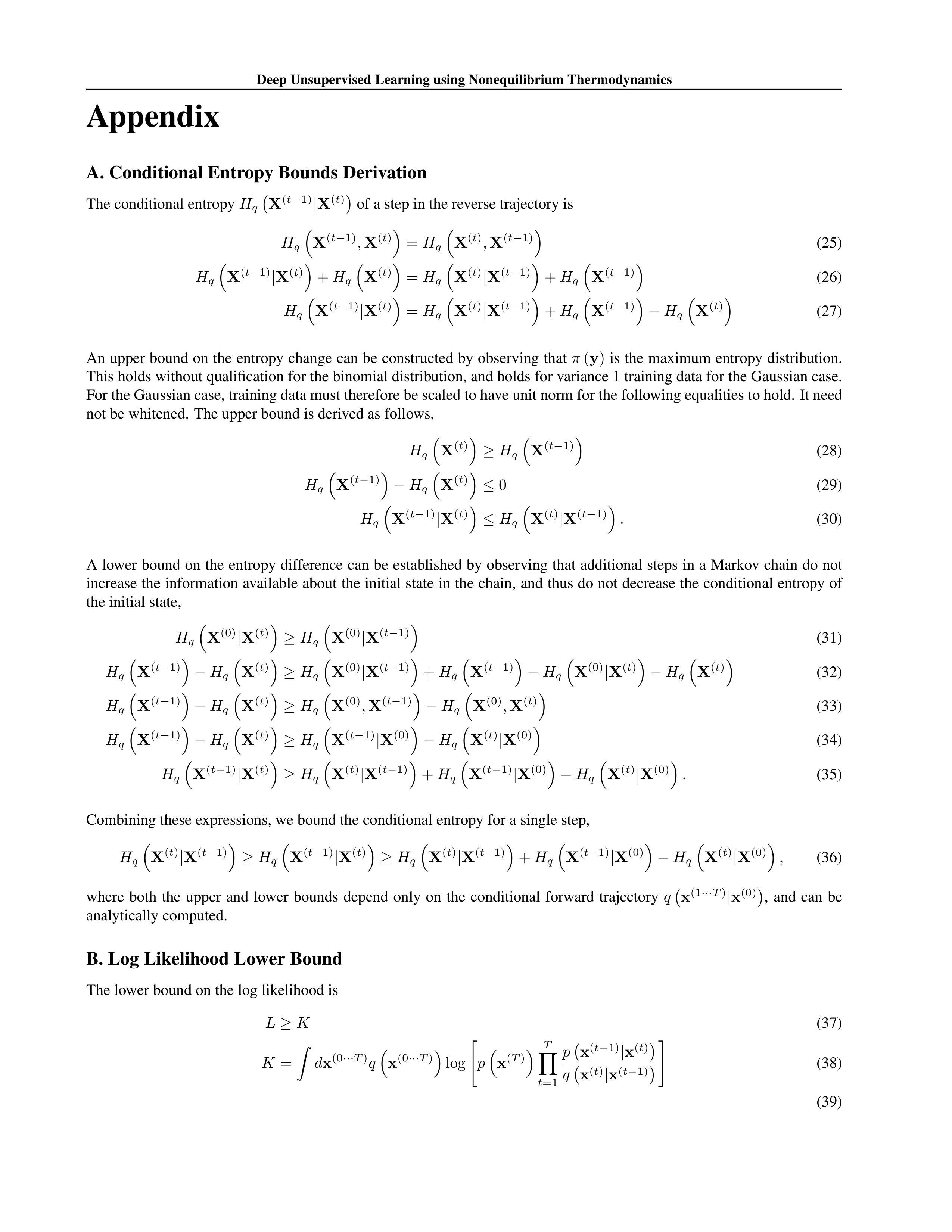
A. Conditional Entropy Bounds Derivation
The conditional entropy
H
q
X
(
t
−
1)
|
X
(
t
)
of a step in the reverse trajectory is
H
q
X
(
t
−
1)
,
X
(
t
)
=
H
q
X
(
t
)
,
X
(
t
−
1)
(25)
H
q
X
(
t
−
1)
|
X
(
t
)
+
H
q
X
(
t
)
=
H
q
X
(
t
)
|
X
(
t
−
1)
+
H
q
X
(
t
−
1)
(26)
H
q
X
(
t
−
1)
|
X
(
t
)
=
H
q
X
(
t
)
|
X
(
t
−
1)
+
H
q
X
(
t
−
1)
−
H
q
X
(
t
)
(27)
An upper bound on the entropy change can be constructed by observing that
π
(
y
)
is the maximum entropy distribution.
This holds without qualification for the binomial distribution, and holds for variance 1 training data for the Gaussian case.
For the Gaussian case, training data must therefore be scaled to have unit norm for the following equalities to hold.
It need
not be whitened.
The upper bound is derived as follows,
H
q
X
(
t
)
≥
H
q
X
(
t
−
1)
(28)
H
q
X
(
t
−
1)
−
H
q
X
(
t
)
≤
0
(29)
H
q
X
(
t
−
1)
|
X
(
t
)
≤
H
q
X
(
t
)
|
X
(
t
−
1)
.
(30)
A lower bound on the
entropy difference can
be established by observing that additional steps in a Markov chain do not
increase the information available about the initial state in the chain,
and thus do not decrease the conditional entropy of
the initial state,
H
q
X
(0)
|
X
(
t
)
≥
H
q
X
(0)
|
X
(
t
−
1)
(31)
H
q
X
(
t
−
1)
−
H
q
X
(
t
)
≥
H
q
X
(0)
|
X
(
t
−
1)
+
H
q
X
(
t
−
1)
−
H
q
X
(0)
|
X
(
t
)
−
H
q
X
(
t
)
(32)
H
q
X
(
t
−
1)
−
H
q
X
(
t
)
≥
H
q
X
(0)
,
X
(
t
−
1)
−
H
q
X
(0)
,
X
(
t
)
(33)
H
q
X
(
t
−
1)
−
H
q
X
(
t
)
≥
H
q
X
(
t
−
1)
|
X
(0)
−
H
q
X
(
t
)
|
X
(0)
(34)
H
q
X
(
t
−
1)
|
X
(
t
)
≥
H
q
X
(
t
)
|
X
(
t
−
1)
+
H
q
X
(
t
−
1)
|
X
(0)
−
H
q
X
(
t
)
|
X
(0)
.
(35)
Combining these expressions, we bound the conditional entropy for a single step,
H
q
X
(
t
)
|
X
(
t
−
1)
≥
H
q
X
(
t
−
1)
|
X
(
t
)
≥
H
q
X
(
t
)
|
X
(
t
−
1)
+
H
q
X
(
t
−
1)
|
X
(0)
−
H
q
X
(
t
)
|
X
(0)
,
(36)
where
both
the
upper
and
lower
bounds
depend
only
on
the
conditional
forward
trajectory
q
x
(1
···
T
)
|
x
(0)
,
and
can
be
analytically computed.
B. Log Likelihood Lower Bound
The lower bound on the log likelihood is
L
≥
K
(37)
K
=
Z
d
x
(0
···
T
)
q
x
(0
···
T
)
log
"
p
x
(
T
)
T
Y
t
=1
p
x
(
t
−
1)
|
x
(
t
)
q
x
(
t
)
|
x
(
t
−
1)
#
(38)
(39)
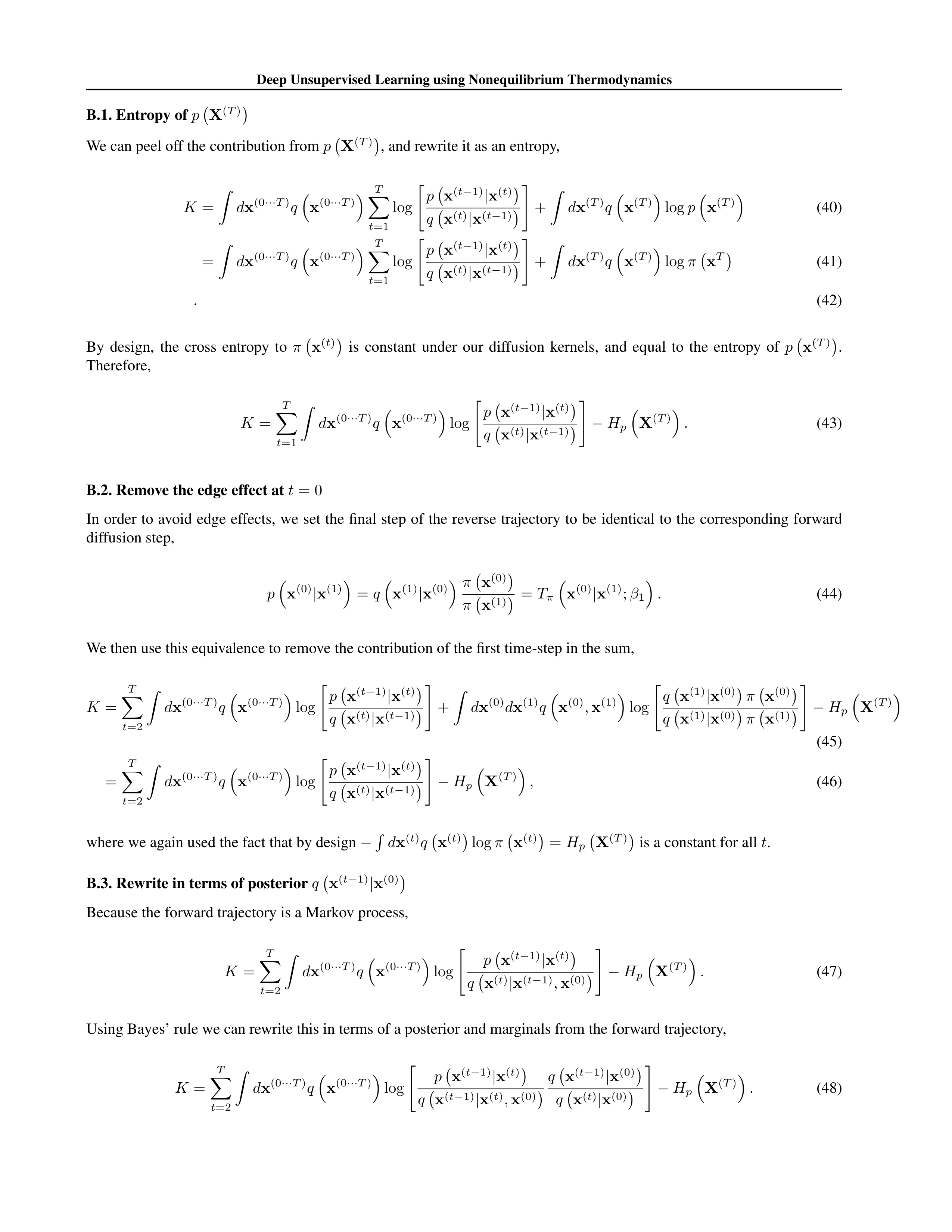
Deep Unsupervised Learning using Nonequilibrium Thermodynamics
B.1. Entropy of
p
X
(
T
)
We can peel off the contribution from
p
X
(
T
)
, and rewrite it as an entropy,
K
=
Z
d
x
(0
···
T
)
q
x
(0
···
T
)
T
X
t
=1
log
"
p
x
(
t
−
1)
|
x
(
t
)
q
x
(
t
)
|
x
(
t
−
1)
#
+
Z
d
x
(
T
)
q
x
(
T
)
log
p
x
(
T
)
(40)
=
Z
d
x
(0
···
T
)
q
x
(0
···
T
)
T
X
t
=1
log
"
p
x
(
t
−
1)
|
x
(
t
)
q
x
(
t
)
|
x
(
t
−
1)
#
+
Z
d
x
(
T
)
q
x
(
T
)
log
π
x
T
(41)
.
(42)
By
design,
the
cross
entropy
to
π
x
(
t
)
is
constant
under
our
diffusion
kernels,
and
equal
to
the
entropy
of
p
x
(
T
)
.
Therefore,
K
=
T
X
t
=1
Z
d
x
(0
···
T
)
q
x
(0
···
T
)
log
"
p
x
(
t
−
1)
|
x
(
t
)
q
x
(
t
)
|
x
(
t
−
1)
#
−
H
p
X
(
T
)
.
(43)
B.2. Remove the edge effect at
t
= 0
In
order
to
avoid
edge
effects,
we
set
the
final
step
of
the
reverse
trajectory
to
be
identical
to
the
corresponding
forward
diffusion step,
p
x
(0)
|
x
(1)
=
q
x
(1)
|
x
(0)
π
x
(0)
π
x
(1)
=
T
π
x
(0)
|
x
(1)
;
β
1
.
(44)
We then use this equivalence to remove the contribution of the first time-step in the sum,
K
=
T
X
t
=2
Z
d
x
(0
···
T
)
q
x
(0
···
T
)
log
"
p
x
(
t
−
1)
|
x
(
t
)
q
x
(
t
)
|
x
(
t
−
1)
#
+
Z
d
x
(0)
d
x
(1)
q
x
(0)
,
x
(1)
log
"
q
x
(1)
|
x
(0)
π
x
(0)
q
x
(1)
|
x
(0)
π
x
(1)
#
−
H
p
X
(
T
)
(45)
=
T
X
t
=2
Z
d
x
(0
···
T
)
q
x
(0
···
T
)
log
"
p
x
(
t
−
1)
|
x
(
t
)
q
x
(
t
)
|
x
(
t
−
1)
#
−
H
p
X
(
T
)
,
(46)
where we again used the fact that by design
−
R
d
x
(
t
)
q
x
(
t
)
log
π
x
(
t
)
=
H
p
X
(
T
)
is a constant for all
t
.
B.3. Rewrite in terms of posterior
q
x
(
t
−
1)
|
x
(0)
Because the forward trajectory is a Markov process,
K
=
T
X
t
=2
Z
d
x
(0
···
T
)
q
x
(0
···
T
)
log
"
p
x
(
t
−
1)
|
x
(
t
)
q
x
(
t
)
|
x
(
t
−
1)
,
x
(0)
#
−
H
p
X
(
T
)
.
(47)
Using Bayes’ rule we can rewrite this in terms of a posterior and marginals from the forward trajectory,
K
=
T
X
t
=2
Z
d
x
(0
···
T
)
q
x
(0
···
T
)
log
"
p
x
(
t
−
1)
|
x
(
t
)
q
x
(
t
−
1)
|
x
(
t
)
,
x
(0)
q
x
(
t
−
1)
|
x
(0)
q
x
(
t
)
|
x
(0)
#
−
H
p
X
(
T
)
.
(48)
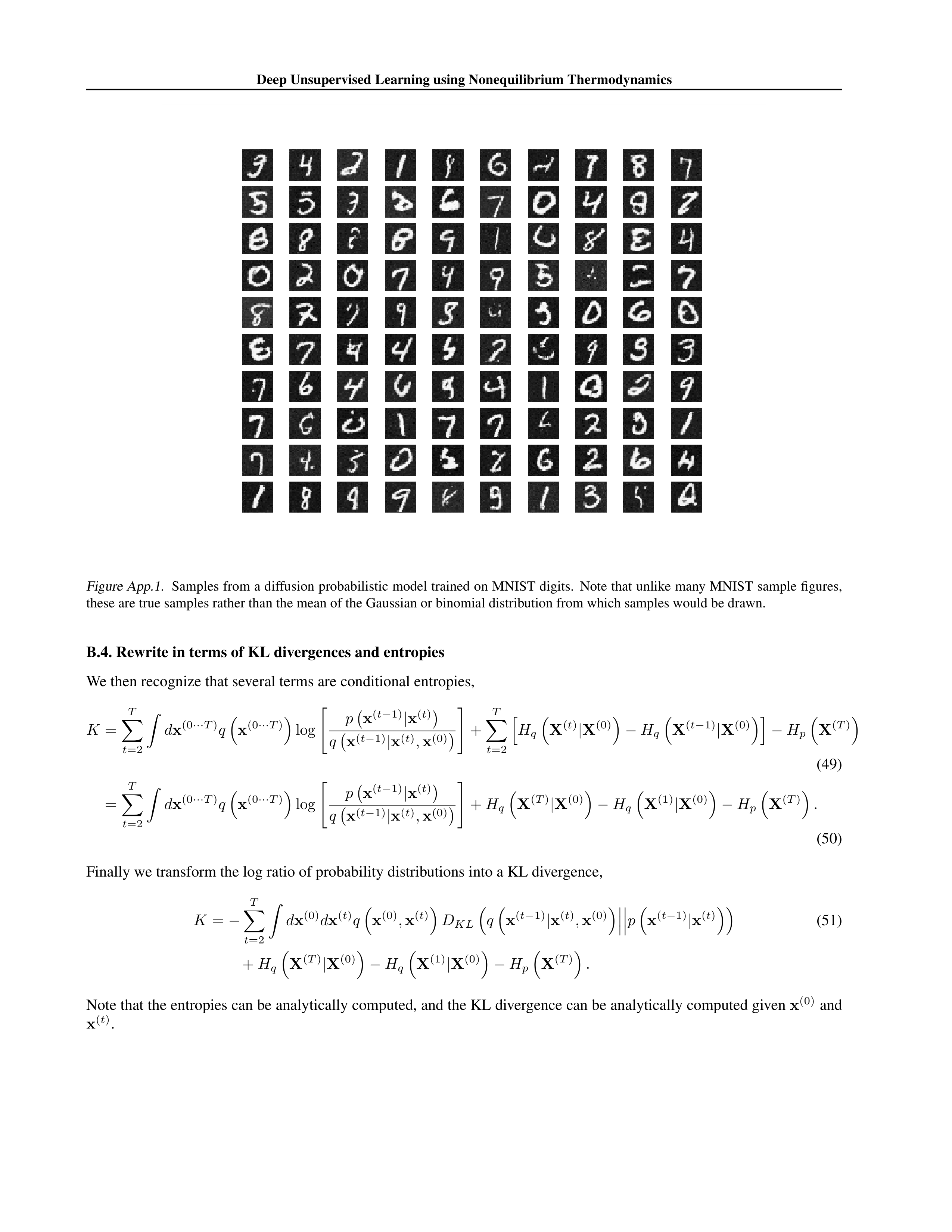


Deep Unsupervised Learning using Nonequilibrium Thermodynamics
Figure App.1.
Samples from a diffusion probabilistic model trained on MNIST digits.
Note that unlike many MNIST sample figures,
these are true samples rather than the mean of the Gaussian or binomial distribution from which samples would be drawn.
B.4. Rewrite in terms of KL divergences and entropies
We then recognize that several terms are conditional entropies,
K
=
T
X
t
=2
Z
d
x
(0
···
T
)
q
x
(0
···
T
)
log
"
p
x
(
t
−
1)
|
x
(
t
)
q
x
(
t
−
1)
|
x
(
t
)
,
x
(0)
#
+
T
X
t
=2
h
H
q
X
(
t
)
|
X
(0)
−
H
q
X
(
t
−
1)
|
X
(0)
i
−
H
p
X
(
T
)
(49)
=
T
X
t
=2
Z
d
x
(0
···
T
)
q
x
(0
···
T
)
log
"
p
x
(
t
−
1)
|
x
(
t
)
q
x
(
t
−
1)
|
x
(
t
)
,
x
(0)
#
+
H
q
X
(
T
)
|
X
(0)
−
H
q
X
(1)
|
X
(0)
−
H
p
X
(
T
)
.
(50)
Finally we transform the log ratio of probability distributions into a KL divergence,
K
=
−
T
X
t
=2
Z
d
x
(0)
d
x
(
t
)
q
x
(0)
,
x
(
t
)
D
KL
q
x
(
t
−
1)
|
x
(
t
)
,
x
(0)
p
x
(
t
−
1)
|
x
(
t
)
(51)
+
H
q
X
(
T
)
|
X
(0)
−
H
q
X
(1)
|
X
(0)
−
H
p
X
(
T
)
.
Note that the entropies can be analytically computed, and the KL divergence can be analytically computed given
x
(0)
and
x
(
t
)
.
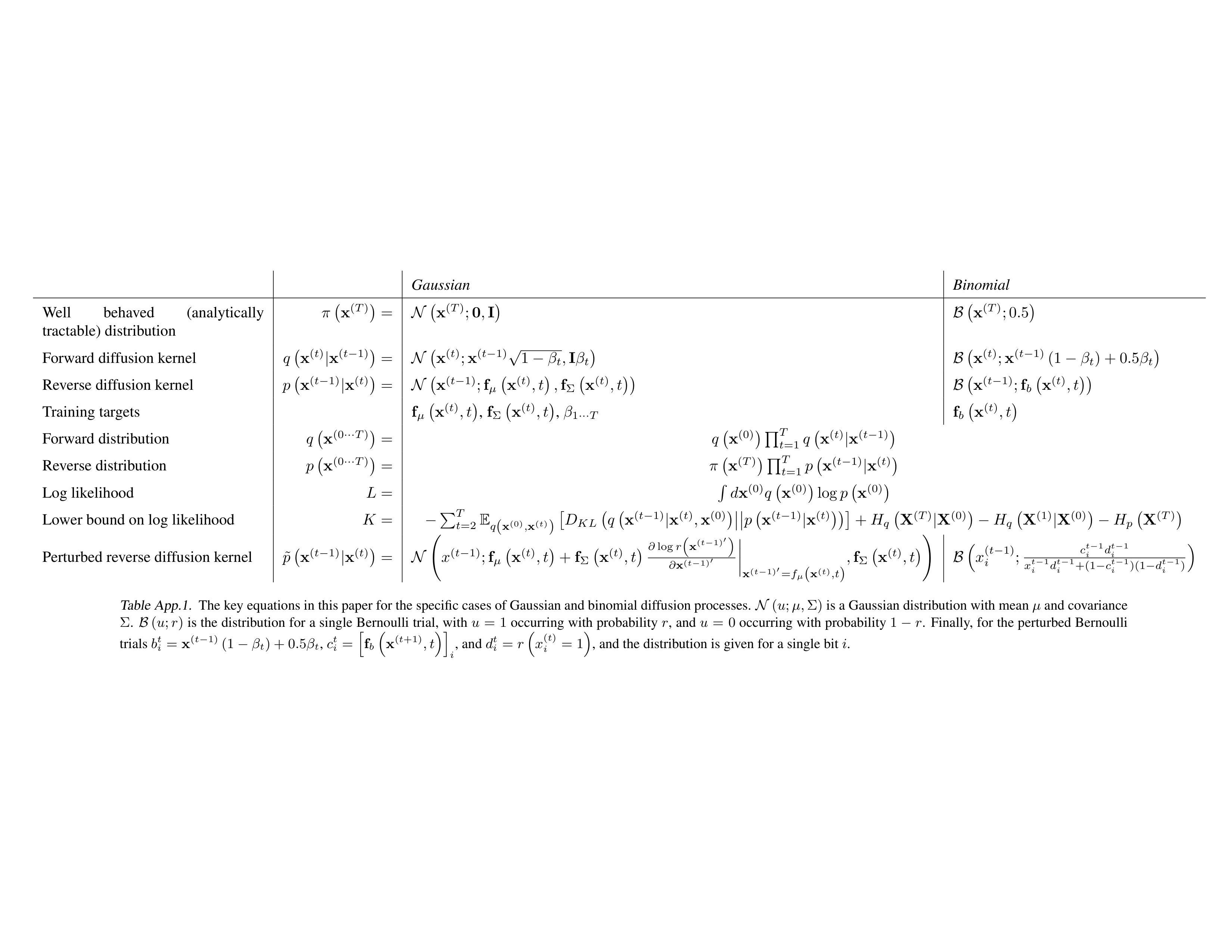
Gaussian
Binomial
Well
behaved
(analytically
tractable) distribution
π
x
(
T
)
=
N
x
(
T
)
;
0
,
I
B
x
(
T
)
; 0
.
5
Forward diffusion kernel
q
x
(
t
)
|
x
(
t
−
1)
=
N
x
(
t
)
;
x
(
t
−
1)
√
1
−
β
t
,
I
β
t
B
x
(
t
)
;
x
(
t
−
1)
(1
−
β
t
) + 0
.
5
β
t
Reverse diffusion kernel
p
x
(
t
−
1)
|
x
(
t
)
=
N
x
(
t
−
1)
;
f
µ
x
(
t
)
, t
,
f
Σ
x
(
t
)
, t
B
x
(
t
−
1)
;
f
b
x
(
t
)
, t
Training targets
f
µ
x
(
t
)
, t
,
f
Σ
x
(
t
)
, t
,
β
1
···
T
f
b
x
(
t
)
, t
Forward distribution
q
x
(0
···
T
)
=
q
x
(0)
Q
T
t
=1
q
x
(
t
)
|
x
(
t
−
1)
Reverse distribution
p
x
(0
···
T
)
=
π
x
(
T
)
Q
T
t
=1
p
x
(
t
−
1)
|
x
(
t
)
Log likelihood
L
=
R
d
x
(0)
q
x
(0)
log
p
x
(0)
Lower bound on log likelihood
K
=
−
P
T
t
=2
E
q
(
x
(0)
,
x
(
t
)
)
D
KL
q
x
(
t
−
1)
|
x
(
t
)
,
x
(0)
p
x
(
t
−
1)
|
x
(
t
)
+
H
q
X
(
T
)
|
X
(0)
−
H
q
X
(1)
|
X
(0)
−
H
p
X
(
T
)
Perturbed reverse diffusion kernel
˜
p
x
(
t
−
1)
|
x
(
t
)
=
N
x
(
t
−
1)
;
f
µ
x
(
t
)
, t
+
f
Σ
x
(
t
)
, t
∂
log
r
x
(
t
−
1)
′
∂
x
(
t
−
1)
′
x
(
t
−
1)
′
=
f
µ
(
x
(
t
)
,t
)
,
f
Σ
x
(
t
)
, t
!
B
x
(
t
−
1)
i
;
c
t
−
1
i
d
t
−
1
i
x
t
−
1
i
d
t
−
1
i
+(1
−
c
t
−
1
i
)(1
−
d
t
−
1
i
)
Table App.1.
The key equations in this paper for the specific cases of Gaussian and binomial diffusion processes.
N
(
u
;
µ,
Σ)
is a Gaussian distribution with mean
µ
and covariance
Σ
.
B
(
u
;
r
)
is the distribution for a single Bernoulli trial, with
u
=
1
occurring with probability
r
, and
u
=
0
occurring with probability
1
−
r
.
Finally, for the perturbed Bernoulli
trials
b
t
i
=
x
(
t
−
1)
(1
−
β
t
) + 0
.
5
β
t
,
c
t
i
=
h
f
b
x
(
t
+1)
, t
i
i
, and
d
t
i
=
r
x
(
t
)
i
= 1
, and the distribution is given for a single bit
i
.
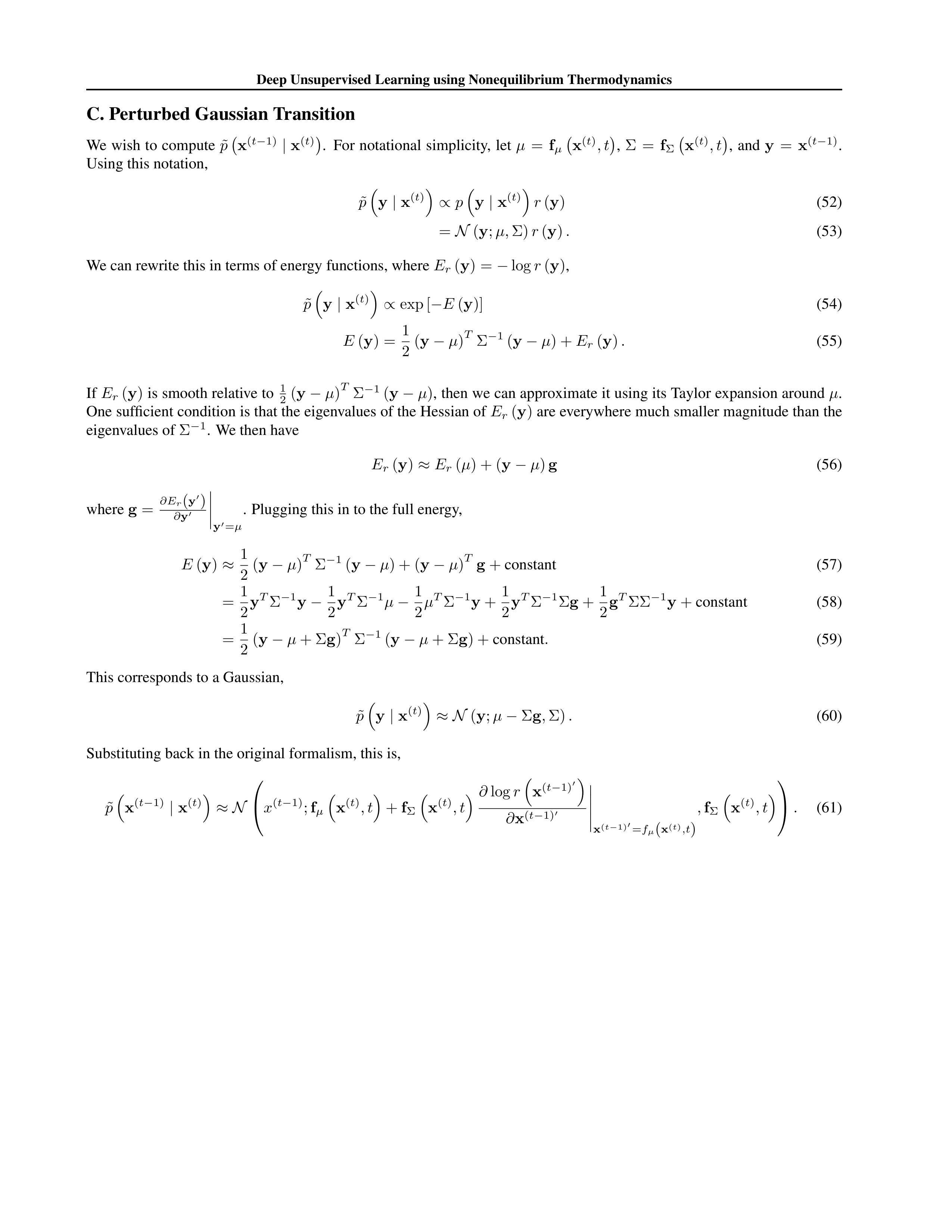
Deep Unsupervised Learning using Nonequilibrium Thermodynamics
C. Perturbed Gaussian Transition
We
wish
to
compute
˜
p
x
(
t
−
1)
|
x
(
t
)
.
For
notational
simplicity,
let
µ
=
f
µ
x
(
t
)
, t
,
Σ
=
f
Σ
x
(
t
)
, t
,
and
y
=
x
(
t
−
1)
.
Using this notation,
˜
p
y
|
x
(
t
)
∝
p
y
|
x
(
t
)
r
(
y
)
(52)
=
N
(
y
;
µ,
Σ)
r
(
y
)
.
(53)
We can rewrite this in terms of energy functions, where
E
r
(
y
) =
−
log
r
(
y
)
,
˜
p
y
|
x
(
t
)
∝
exp [
−
E
(
y
)]
(54)
E
(
y
) =
1
2
(
y
−
µ
)
T
Σ
−
1
(
y
−
µ
) +
E
r
(
y
)
.
(55)
If
E
r
(
y
)
is smooth relative to
1
2
(
y
−
µ
)
T
Σ
−
1
(
y
−
µ
)
, then we can approximate it using its Taylor expansion around
µ
.
One sufficient condition is that the eigenvalues of the Hessian of
E
r
(
y
)
are everywhere much smaller magnitude than the
eigenvalues of
Σ
−
1
.
We then have
E
r
(
y
)
≈
E
r
(
µ
) + (
y
−
µ
)
g
(56)
where
g
=
∂E
r
(
y
′
)
∂
y
′
y
′
=
µ
.
Plugging this in to the full energy,
E
(
y
)
≈
1
2
(
y
−
µ
)
T
Σ
−
1
(
y
−
µ
) + (
y
−
µ
)
T
g
+
constant
(57)
=
1
2
y
T
Σ
−
1
y
−
1
2
y
T
Σ
−
1
µ
−
1
2
µ
T
Σ
−
1
y
+
1
2
y
T
Σ
−
1
Σ
g
+
1
2
g
T
ΣΣ
−
1
y
+
constant
(58)
=
1
2
(
y
−
µ
+ Σ
g
)
T
Σ
−
1
(
y
−
µ
+ Σ
g
) +
constant
.
(59)
This corresponds to a Gaussian,
˜
p
y
|
x
(
t
)
≈N
(
y
;
µ
−
Σ
g
,
Σ)
.
(60)
Substituting back in the original formalism, this is,
˜
p
x
(
t
−
1)
|
x
(
t
)
≈N
x
(
t
−
1)
;
f
µ
x
(
t
)
, t
+
f
Σ
x
(
t
)
, t
∂
log
r
x
(
t
−
1)
′
∂
x
(
t
−
1)
′
x
(
t
−
1)
′
=
f
µ
(
x
(
t
)
,t
)
,
f
Σ
x
(
t
)
, t
.
(61)
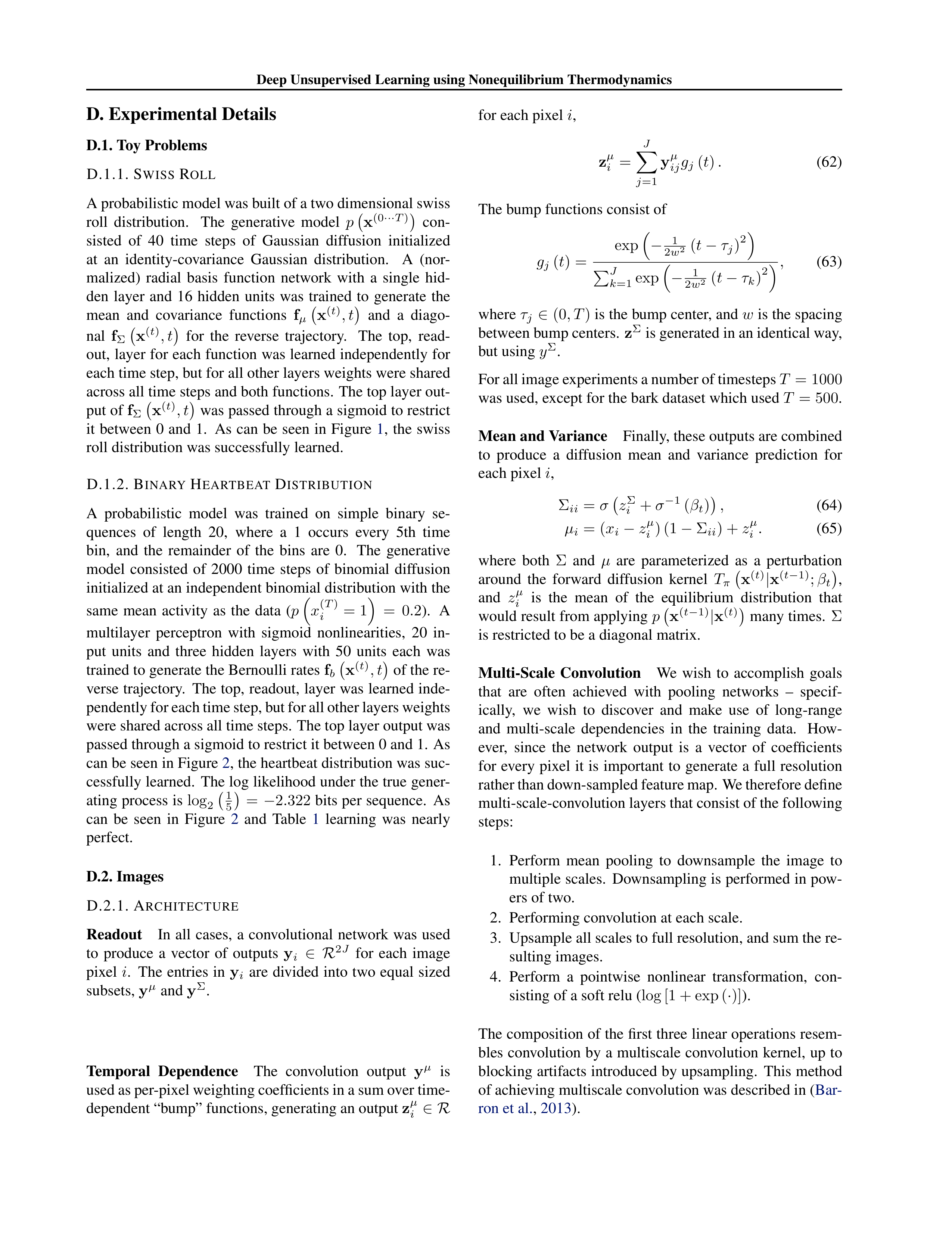
Deep Unsupervised Learning using Nonequilibrium Thermodynamics
D. Experimental Details
D.1. Toy Problems
D.1.1. S
WISS
R
OLL
A probabilistic model was built of a two dimensional swiss
roll
distribution.
The
generative
model
p
x
(0
···
T
)
con-
sisted
of
40
time
steps
of
Gaussian
diffusion
initialized
at
an
identity-covariance
Gaussian
distribution.
A
(nor-
malized)
radial
basis
function
network
with
a
single
hid-
den
layer
and
16
hidden
units
was
trained
to
generate
the
mean
and
covariance
functions
f
µ
x
(
t
)
, t
and
a
diago-
nal
f
Σ
x
(
t
)
, t
for
the
reverse
trajectory.
The
top,
read-
out, layer for each function was learned independently for
each time step, but for all other layers weights were shared
across all time steps and both functions.
The top layer out-
put of
f
Σ
x
(
t
)
, t
was passed through a sigmoid to restrict
it
between
0
and
1.
As
can
be
seen
in
Figure
1
,
the
swiss
roll distribution was successfully learned.
D.1.2. B
INARY
H
EARTBEAT
D
ISTRIBUTION
A
probabilistic
model
was
trained
on
simple
binary
se-
quences
of
length
20,
where
a
1
occurs
every
5th
time
bin,
and
the
remainder
of
the
bins
are
0.
The
generative
model
consisted
of
2000
time
steps
of
binomial
diffusion
initialized at an independent binomial distribution with the
same
mean
activity
as
the
data
(
p
x
(
T
)
i
= 1
=
0
.
2
).
A
multilayer
perceptron
with
sigmoid
nonlinearities,
20
in-
put
units
and
three
hidden
layers
with
50
units
each
was
trained to generate the Bernoulli rates
f
b
x
(
t
)
, t
of the re-
verse trajectory.
The top,
readout,
layer was learned inde-
pendently for each time step, but for all other layers weights
were shared across all time steps.
The top layer output was
passed through a sigmoid to restrict it between 0 and 1.
As
can be seen in Figure
2
, the heartbeat distribution was suc-
cessfully learned.
The log likelihood under the true gener-
ating process is
log
2
1
5
=
−
2
.
322
bits per sequence.
As
can
be
seen
in
Figure
2
and
Table
1
learning
was
nearly
perfect.
D.2. Images
D.2.1. A
RCHITECTURE
Readout
In
all
cases,
a
convolutional
network
was
used
to
produce
a
vector
of
outputs
y
i
∈R
2
J
for
each
image
pixel
i
.
The
entries
in
y
i
are
divided
into
two
equal
sized
subsets,
y
µ
and
y
Σ
.
Temporal
Dependence
The
convolution
output
y
µ
is
used as per-pixel weighting coefficients in a sum over time-
dependent “bump” functions, generating an output
z
µ
i
∈R
for each pixel
i
,
z
µ
i
=
J
X
j
=1
y
µ
ij
g
j
(
t
)
.
(62)
The bump functions consist of
g
j
(
t
) =
exp
−
1
2
w
2
(
t
−
τ
j
)
2
P
J
k
=1
exp
−
1
2
w
2
(
t
−
τ
k
)
2
,
(63)
where
τ
j
∈
(0
, T
)
is the bump center, and
w
is the spacing
between bump centers.
z
Σ
is generated in an identical way,
but using
y
Σ
.
For all image experiments a number of timesteps
T
= 1000
was used, except for the bark dataset which used
T
= 500
.
Mean and Variance
Finally, these outputs are combined
to
produce
a
diffusion
mean
and
variance
prediction
for
each pixel
i
,
Σ
ii
=
σ
z
Σ
i
+
σ
−
1
(
β
t
)
,
(64)
µ
i
= (
x
i
−
z
µ
i
) (1
−
Σ
ii
) +
z
µ
i
.
(65)
where
both
Σ
and
µ
are
parameterized
as
a
perturbation
around
the
forward
diffusion
kernel
T
π
x
(
t
)
|
x
(
t
−
1)
;
β
t
,
and
z
µ
i
is
the
mean
of
the
equilibrium
distribution
that
would result from applying
p
x
(
t
−
1)
|
x
(
t
)
many times.
Σ
is restricted to be a diagonal matrix.
Multi-Scale
Convolution
We
wish
to
accomplish
goals
that
are
often
achieved
with
pooling
networks
–
specif-
ically,
we
wish
to
discover
and
make
use
of
long-range
and
multi-scale
dependencies
in
the
training
data.
How-
ever,
since
the
network
output
is
a
vector
of
coefficients
for
every
pixel
it
is
important
to
generate
a
full
resolution
rather than down-sampled feature map. We therefore define
multi-scale-convolution layers that consist of the following
steps:
1.
Perform
mean
pooling
to
downsample
the
image
to
multiple scales.
Downsampling is performed in pow-
ers of two.
2.
Performing convolution at each scale.
3.
Upsample all scales to full resolution, and sum the re-
sulting images.
4.
Perform
a
pointwise
nonlinear
transformation,
con-
sisting of a soft relu (
log [1 + exp (
·
)]
).
The composition of the first three linear operations resem-
bles convolution by a multiscale convolution kernel,
up to
blocking artifacts introduced by upsampling.
This method
of achieving multiscale convolution was described in (
Bar-
ron et al.
,
2013
).
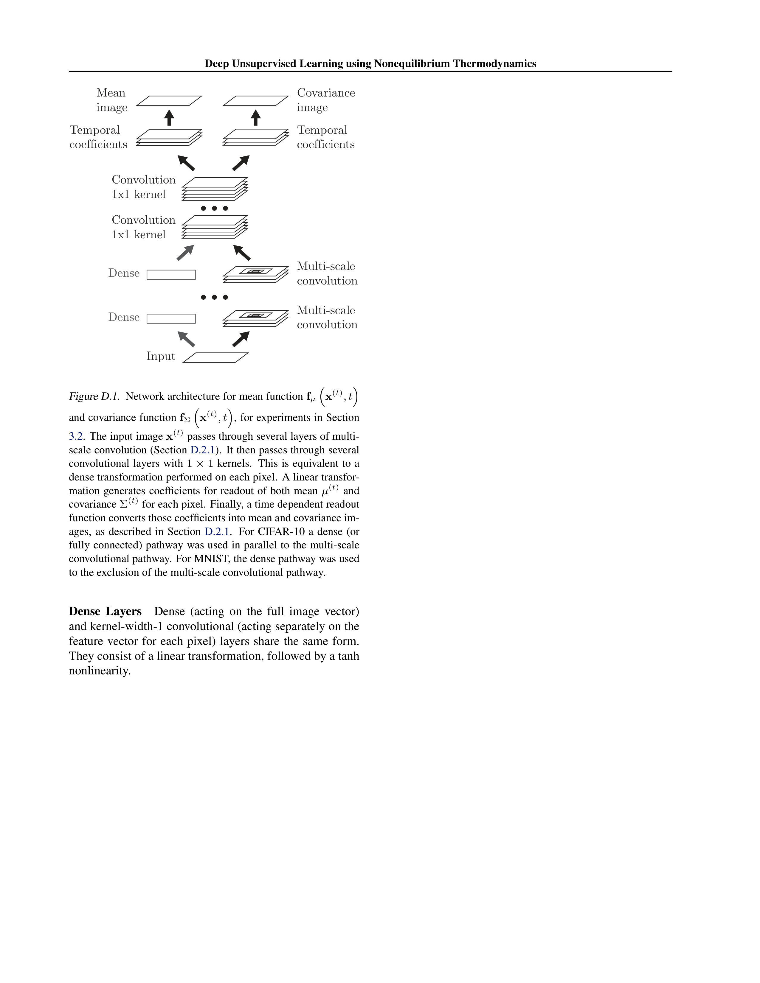
Deep Unsupervised Learning using Nonequilibrium Thermodynamics
Input
Dense
Multi-scale
convolution
Convolution
1x1 kernel
Temporal
coefficients
Temporal
coefficients
Dense
Multi-scale
convolution
Mean
image
Covariance
image
Convolution
1x1 kernel
Figure D.1.
Network architecture for mean function
f
µ
x
(
t
)
, t
and covariance function
f
Σ
x
(
t
)
, t
,
for experiments in Section
3.2
.
The input image
x
(
t
)
passes through several layers of multi-
scale convolution (Section
D.2.1
).
It then passes through several
convolutional
layers
with
1
×
1
kernels.
This
is
equivalent
to
a
dense transformation performed on each pixel.
A linear transfor-
mation
generates
coefficients
for
readout
of
both
mean
µ
(
t
)
and
covariance
Σ
(
t
)
for each pixel.
Finally, a time dependent readout
function converts those coefficients into mean and covariance im-
ages,
as
described
in
Section
D.2.1
.
For
CIFAR-10
a
dense
(or
fully
connected)
pathway
was
used
in
parallel
to
the
multi-scale
convolutional pathway.
For MNIST, the dense pathway was used
to the exclusion of the multi-scale convolutional pathway.
Dense
Layers
Dense
(acting
on
the
full
image
vector)
and kernel-width-1 convolutional (acting separately on the
feature
vector
for
each
pixel)
layers
share
the
same
form.
They consist of a linear transformation, followed by a tanh
nonlinearity.