
Scaling Laws for Neural Language Models
Jared Kaplan
∗
Johns Hopkins University, OpenAI
jaredk@jhu.edu
Sam McCandlish
∗
OpenAI
sam@openai.com
Tom Henighan
OpenAI
henighan@openai.com
Tom B. Brown
OpenAI
tom@openai.com
Benjamin Chess
OpenAI
bchess@openai.com
Rewon Child
OpenAI
rewon@openai.com
Scott Gray
OpenAI
scott@openai.com
Alec Radford
OpenAI
alec@openai.com
Jeffrey Wu
OpenAI
jeffwu@openai.com
Dario Amodei
OpenAI
damodei@openai.com
Abstract
We study empirical scaling laws for language model performance on the cross-entropy loss.
The
loss
scales
as
a
power-law
with
model
size,
dataset
size,
and
the
amount
of
compute
used for training, with some trends spanning more than seven orders of magnitude.
Other
architectural
details
such
as
network
width
or
depth
have
minimal
effects
within
a
wide
range. Simple equations govern the dependence of overfitting on model/dataset size and the
dependence of training speed on model size.
These relationships allow us to determine the
optimal allocation of a fixed compute budget. Larger models are significantly more sample-
efficient, such that optimally compute-efficient training involves training very large models
on a relatively modest amount of data and stopping significantly before convergence.
∗
Equal contribution.
Contributions:
Jared
Kaplan
and
Sam
McCandlish
led
the
research.
Tom
Henighan
contributed
the
LSTM
ex-
periments.
Tom
Brown,
Rewon
Child,
and
Scott
Gray,
and
Alec
Radford
developed
the
optimized
Transformer
implementation.
Jeff
Wu,
Benjamin
Chess,
and
Alec
Radford
developed
the
text
datasets.
Dario
Amodei
provided
guidance throughout the project.
arXiv:2001.08361v1 [cs.LG] 23 Jan 2020
Contents
1
Introduction
2
2
Background and Methods
6
3
Empirical Results and Basic Power Laws
7
4
Charting the Infinite Data Limit and Overfitting
10
5
Scaling Laws with Model Size and Training Time
12
6
Optimal Allocation of the Compute Budget
14
7
Related Work
18
8
Discussion
18
Appendices
20
A
Summary of Power Laws
20
B
Empirical Model of Compute-Efficient Frontier
20
C
Caveats
22
D
Supplemental Figures
23
1
Introduction
Language
provides
a
natural
domain
for
the
study
of
artificial
intelligence,
as
the
vast
majority
of
reason-
ing
tasks
can
be
efficiently
expressed
and
evaluated
in
language,
and
the
world’s
text
provides
a
wealth
of
data for unsupervised learning via generative modeling. Deep learning has recently seen rapid progress in lan-
guage modeling, with state of the art models [RNSS18, DCLT18, YDY
+
19, LOG
+
19, RSR
+
19] approaching
human-level
performance
on
many
specific tasks
[WPN
+
19],
including
the
composition of
coherent multi-
paragraph prompted text samples [RWC
+
19].
One might expect language modeling performance to depend on model architecture, the size of neural models,
the computing power used to train them, and the data available for this training process.
In this work we will
empirically
investigate
the
dependence
of
language
modeling
loss
on
all
of
these
factors,
focusing
on
the
Transformer architecture [VSP
+
17, LSP
+
18].
The high ceiling and low floor for performance on language
tasks allows us to study trends over more than seven orders of magnitude in scale.
Throughout we will observe precise power-law scalings for performance as a function of training time, con-
text length, dataset size, model size, and compute budget.
1.1
Summary
Our key findings for Transformer language models are are as follows:
2
Here we display predicted compute when using a sufficiently small batch size.
See Figure 13 for comparison to the
purely empirical data.
2
Dataset Size
tokens
Parameters
non-embedding
Compute
PF-days, non-embedding
Test Loss
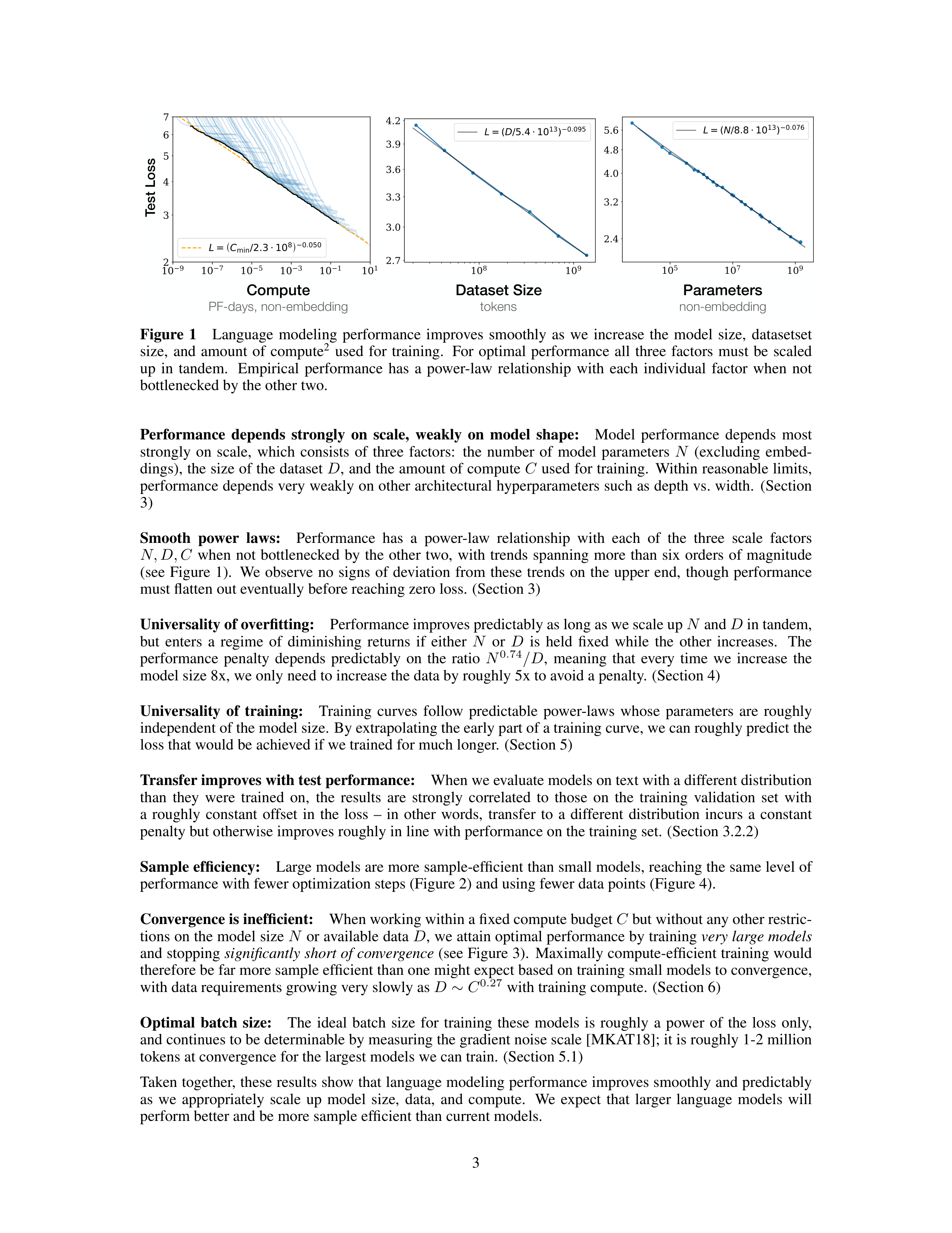
Figure
1
Language
modeling
performance
improves
smoothly
as
we
increase
the
model
size,
datasetset
size,
and
amount
of
compute
2
used
for
training.
For
optimal
performance
all
three
factors
must
be
scaled
up
in
tandem.
Empirical
performance
has
a
power-law
relationship
with
each
individual
factor
when
not
bottlenecked by the other two.
Performance
depends
strongly
on
scale,
weakly
on
model
shape:
Model
performance
depends
most
strongly
on
scale,
which
consists
of
three
factors:
the
number
of
model
parameters
N
(excluding
embed-
dings), the size of the dataset
D
, and the amount of compute
C
used for training.
Within reasonable limits,
performance depends very weakly on other architectural hyperparameters such as depth vs. width.
(Section
3)
Smooth
power
laws:
Performance
has
a
power-law
relationship
with
each
of
the
three
scale
factors
N, D, C
when
not
bottlenecked
by
the
other
two,
with
trends
spanning
more
than
six
orders
of
magnitude
(see
Figure
1).
We
observe
no
signs
of
deviation
from
these
trends
on
the
upper
end,
though
performance
must flatten out eventually before reaching zero loss.
(Section 3)
Universality of overfitting:
Performance improves predictably as long as we scale up
N
and
D
in tandem,
but
enters
a
regime
of
diminishing
returns
if
either
N
or
D
is
held
fixed
while
the
other
increases.
The
performance
penalty
depends
predictably
on
the
ratio
N
0
.
74
/D
,
meaning
that
every
time
we
increase
the
model size 8x, we only need to increase the data by roughly 5x to avoid a penalty.
(Section 4)
Universality
of
training:
Training
curves
follow
predictable
power-laws
whose
parameters
are
roughly
independent of the model size.
By extrapolating the early part of a training curve, we can roughly predict the
loss that would be achieved if we trained for much longer.
(Section 5)
Transfer improves with test performance:
When we evaluate models on text with a different distribution
than
they
were
trained
on,
the
results
are
strongly
correlated
to
those
on
the
training
validation
set
with
a
roughly
constant
offset
in
the
loss
–
in
other
words,
transfer
to
a
different
distribution
incurs
a
constant
penalty but otherwise improves roughly in line with performance on the training set.
(Section 3.2.2)
Sample efficiency:
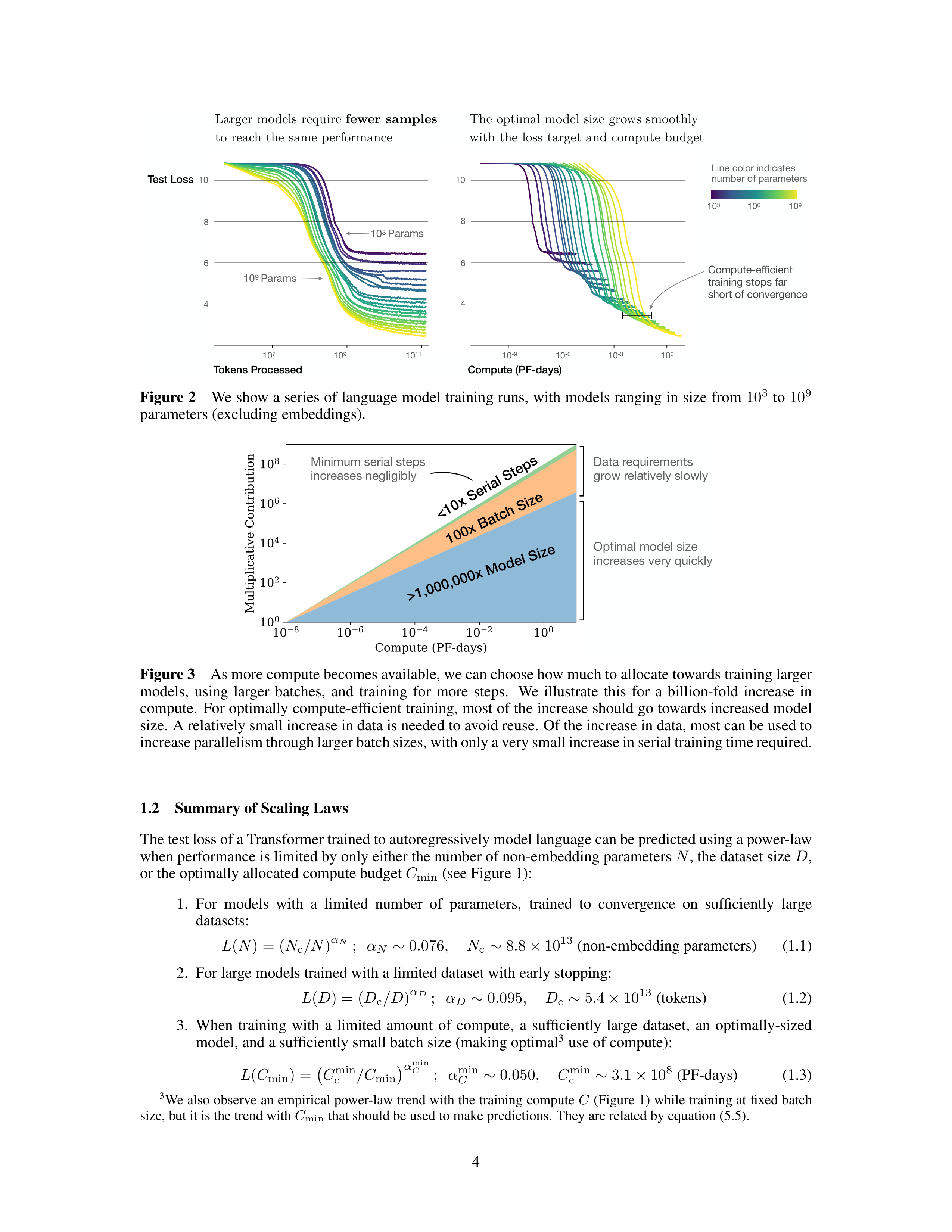
Large models are more sample-efficient than small models, reaching the same level of
performance with fewer optimization steps (Figure 2) and using fewer data points (Figure 4).
Convergence is inefficient:
When working within a fixed compute budget
C
but without any other restric-
tions on the model size
N
or available data
D
, we attain optimal performance by training
very large models
and stopping
significantly short of convergence
(see Figure 3).
Maximally compute-efficient training would
therefore be far more sample efficient than one might expect based on training small models to convergence,
with data requirements growing very slowly as
D
∼
C
0
.
27
with training compute.
(Section 6)
Optimal
batch
size:
The
ideal
batch
size
for
training
these
models
is
roughly
a
power
of
the
loss
only,
and continues to be determinable by measuring the gradient noise scale [MKAT18]; it is roughly 1-2 million
tokens at convergence for the largest models we can train.
(Section 5.1)
Taken together, these results show that language modeling performance improves smoothly and predictably
as
we
appropriately
scale
up
model
size,
data,
and
compute.
We
expect
that
larger
language
models
will
perform better and be more sample efficient than current models.
3

Larger models require
fewer samples
to reach the same performance
10
8
6
4
The optimal model size grows smoothly
with the loss target and compute budget
Line color indicates
number of parameters
10
7
10
9
10
11
Tokens Processed
Compute (PF-days)
10
-9
10
-6
10
-3
10
0
Test Loss
Compute-efficient
training stops far
short of convergence
10
3
10
9
10
6
10
3
Params
10
9
Params
10
8
6
4
Figure 2
We show a series of language model training runs, with models ranging in size from
10
3
to
10
9
parameters (excluding embeddings).
100x Batch Size
<10x Serial Steps
>1,000,000x Model Size
Data requirements
grow relatively slowly
Optimal model size
increases very quickly
Minimum serial steps
increases negligibly
Figure 3
As more compute becomes available, we can choose how much to allocate towards training larger
models,
using
larger
batches,
and
training
for
more
steps.
We
illustrate
this
for
a
billion-fold
increase
in
compute.
For optimally compute-efficient training, most of the increase should go towards increased model
size.
A relatively small increase in data is needed to avoid reuse.
Of the increase in data, most can be used to
increase parallelism through larger batch sizes, with only a very small increase in serial training time required.
1.2
Summary of Scaling Laws
The test loss of a Transformer trained to autoregressively model language can be predicted using a power-law
when performance is limited by only either the number of non-embedding parameters
N
, the dataset size
D
,
or the optimally allocated compute budget
C
min
(see Figure 1):
1.
For
models
with
a
limited
number
of
parameters,
trained
to
convergence
on
sufficiently
large
datasets:
L
(
N
) = (
N
c
/N
)
α
N
;
α
N
∼
0
.
076
,
N
c
∼
8
.
8
×
10
13
(non-embedding parameters)
(1.1)
2.
For large models trained with a limited dataset with early stopping:
L
(
D
) = (
D
c
/D
)
α
D
;
α
D
∼
0
.
095
,
D
c
∼
5
.
4
×
10
13
(tokens)
(1.2)
3.
When
training
with
a
limited
amount
of
compute,
a
sufficiently
large
dataset,
an
optimally-sized
model, and a sufficiently small batch size (making optimal
3
use of compute):
L
(
C
min
) =
C
min
c
/C
min
α
min
C
;
α
min
C
∼
0
.
050
,
C
min
c
∼
3
.
1
×
10
8
(PF-days)
(1.3)
3
We also observe an empirical power-law trend with the training compute
C
(Figure 1) while training at fixed batch
size, but it is the trend with
C
min
that should be used to make predictions.
They are related by equation (5.5).
4

10
7
10
8
10
9
10
10
Tokens in Dataset
2.5
3.0
3.5
4.0
4.5
Loss
Loss vs Model and Dataset Size
Params
708M
302M
85M
3M
25M
393.2K
10
4
10
5
Estimated
S
min
2.4
2.8
3.2
3.6
4.0
4.4
Loss
Loss vs Model Size and Training Steps
10
6
10
7
10
8
Parameters (non-embed)
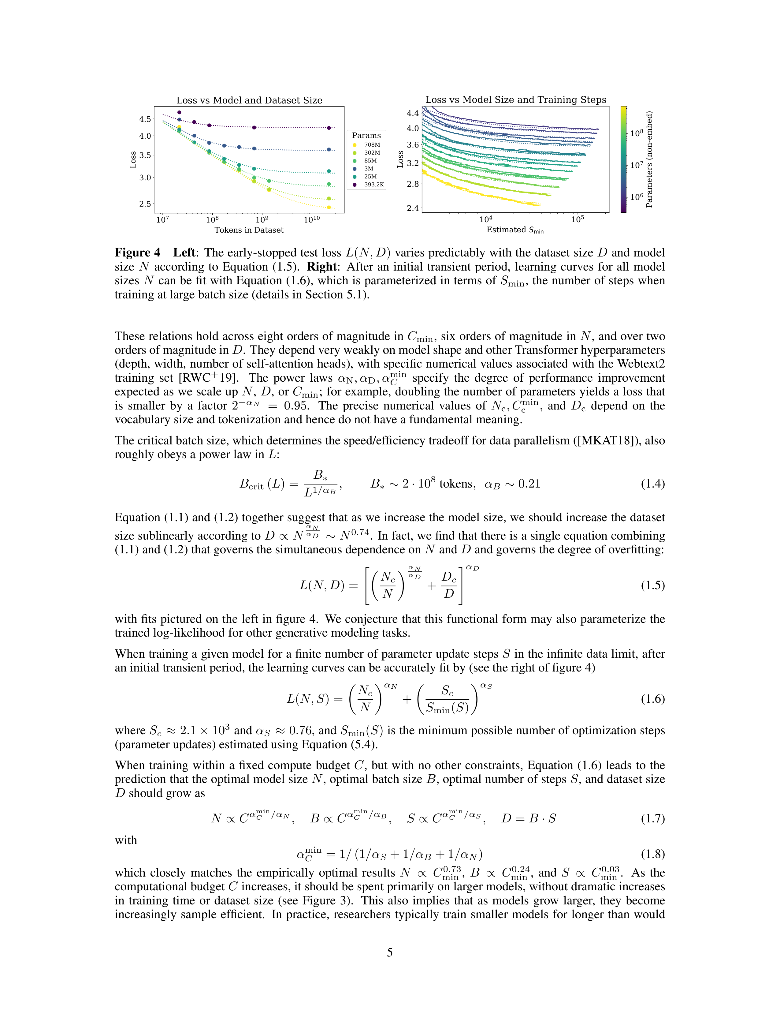
Figure 4
Left
:
The early-stopped test loss
L
(
N, D
)
varies predictably with the dataset size
D
and model
size
N
according
to
Equation
(1.5).
Right
:
After
an
initial
transient
period,
learning
curves
for
all
model
sizes
N
can be fit with Equation (1.6),
which is parameterized in terms of
S
min
,
the number of steps when
training at large batch size (details in Section 5.1).
These relations hold across eight orders of magnitude in
C
min
, six orders of magnitude in
N
, and over two
orders of magnitude in
D
.
They depend very weakly on model shape and other Transformer hyperparameters
(depth, width, number of self-attention heads), with specific numerical values associated with the Webtext2
training
set
[RWC
+
19].
The
power
laws
α
N
, α
D
, α
min
C
specify
the
degree
of
performance
improvement
expected as we scale up
N
,
D
,
or
C
min
;
for example,
doubling the number of parameters yields a loss that
is
smaller
by
a
factor
2
−
α
N
=
0
.
95
.
The
precise
numerical
values
of
N
c
, C
min
c
,
and
D
c
depend
on
the
vocabulary size and tokenization and hence do not have a fundamental meaning.
The critical batch size, which determines the speed/efficiency tradeoff for data parallelism ([MKAT18]), also
roughly obeys a power law in
L
:
B
crit
(
L
) =
B
∗
L
1
/α
B
,
B
∗
∼
2
·
10
8
tokens
,
α
B
∼
0
.
21
(1.4)
Equation (1.1) and (1.2) together suggest that as we increase the model size, we should increase the dataset
size sublinearly according to
D
∝
N
αN
αD
∼
N
0
.
74
.
In fact, we find that there is a single equation combining
(1.1) and (1.2) that governs the simultaneous dependence on
N
and
D
and governs the degree of overfitting:
L
(
N, D
) =
"
N
c
N
α
N
αD
+
D
c
D
#
α
D
(1.5)
with fits pictured on the left in figure 4.
We conjecture that this functional form may also parameterize the
trained log-likelihood for other generative modeling tasks.
When training a given model for a finite number of parameter update steps
S
in the infinite data limit, after
an initial transient period, the learning curves can be accurately fit by (see the right of figure 4)
L
(
N, S
) =
N
c
N
α
N
+
S
c
S
min
(
S
)
α
S
(1.6)
where
S
c
≈
2
.
1
×
10
3
and
α
S
≈
0
.
76
, and
S
min
(
S
)
is the minimum possible number of optimization steps
(parameter updates) estimated using Equation (5.4).
When
training
within
a
fixed
compute
budget
C
,
but
with
no
other
constraints,
Equation
(1.6)
leads
to
the
prediction that the optimal model size
N
, optimal batch size
B
, optimal number of steps
S
, and dataset size
D
should grow as
N
∝
C
α
min
C
/α
N
,
B
∝
C
α
min
C
/α
B
,
S
∝
C
α
min
C
/α
S
,
D
=
B
·
S
(1.7)
with
α
min
C
= 1
/
(1
/α
S
+ 1
/α
B
+ 1
/α
N
)
(1.8)
which
closely
matches
the
empirically
optimal
results
N
∝
C
0
.
73
min
,
B
∝
C
0
.
24
min
,
and
S
∝
C
0
.
03
min
.
As
the
computational budget
C
increases, it should be spent primarily on larger models, without dramatic increases
in
training
time
or
dataset
size
(see
Figure
3).
This
also
implies
that
as
models
grow
larger,
they
become
increasingly
sample
efficient.
In
practice,
researchers
typically
train
smaller
models
for
longer
than
would
5
be
maximally
compute-efficient
because
of
hardware
constraints.
Optimal
performance
depends
on
total
compute as a power law (see Equation (1.3)).
We provide some basic theoretical motivation for Equation (1.5), an analysis of learning curve fits and their
implications for training time, and a breakdown of our results per token.
We also make some brief compar-
isons to LSTMs and recurrent Transformers [DGV
+
18].
1.3
Notation
We use the following notation:
•
L
– the cross entropy loss in nats.
Typically it will be averaged over the tokens in a context, but in
some cases we report the loss for specific tokens within the context.
•
N
– the number of model parameters,
excluding all vocabulary and positional embeddings
•
C
≈
6
NBS
– an estimate of the total non-embedding training compute, where
B
is the batch size,
and
S
is the number of training steps (ie parameter updates).
We quote numerical values in PF-days,
where one PF-day
= 10
15
×
24
×
3600 = 8
.
64
×
10
19
floating point operations.
•
D
– the dataset size in tokens
•
B
crit
–
the
critical
batch
size
[MKAT18],
defined
and
discussed
in
Section
5.1.
Training
at
the
critical batch size provides a roughly optimal compromise between time and compute efficiency.
•
C
min
–
an
estimate
of
the
minimum
amount
of
non-embedding
compute
to
reach
a
given
value
of
the loss.
This is the training compute that would be used if the model were trained at a batch size
much less than the critical batch size.
•
S
min
– an estimate of the minimal number of training steps needed to reach a given value of the loss.
This is also the number of training steps that would be used if the model were trained at a batch size
much greater than the critical batch size.
•
α
X
– power-law exponents for the scaling of the loss as
L
(
X
)
∝
1
/X
α
X
where
X
can be any of
N, D, C, S, B, C
min
.
2
Background and Methods
We train language models on WebText2, an extended version of the WebText [RWC
+
19] dataset, tokenized
using
byte-pair
encoding
[SHB15]
with
a
vocabulary
size
n
vocab
=
50257
.
We
optimize
the
autoregres-
sive log-likelihood (i.e.
cross-entropy loss) averaged over a 1024-token context, which is also our principal
performance
metric.
We
record
the
loss
on
the
WebText2
test
distribution
and
on
a
selection
of
other
text
distributions.
We primarily
train decoder-only [LSP
+
18, RNSS18] Transformer [VSP
+
17] models,
though
we also train LSTM models and Universal Transformers [DGV
+
18] for comparison.
2.1
Parameter and Compute Scaling of Transformers
We parameterize the Transformer architecture using hyperparameters
n
layer
(number of layers),
d
model
(di-
mension of the residual stream),
d
ff
(dimension of the intermediate feed-forward layer),
d
attn
(dimension of
the attention output), and
n
heads
(number of attention heads per layer).
We include
n
ctx
tokens in the input
context, with
n
ctx
= 1024
except where otherwise noted.
We use
N
to denote the model size, which we define as the number of
non-embedding
parameters
N
≈
2
d
model
n
layer
(2
d
attn
+
d
ff
)
= 12
n
layer
d
2
model
with the standard
d
attn
=
d
ff
/
4 =
d
model
(2.1)
where we have excluded biases and other sub-leading terms.
Our models also have
n
vocab
d
model
parameters
in
an
embedding
matrix,
and
use
n
ctx
d
model
parameters
for
positional
embeddings,
but
we
do
not
include
these when discussing the ‘model size’
N
; we will see that this produces significantly cleaner scaling laws.
Evaluating a forward pass of the Transformer involves roughly
C
forward
≈
2
N
+ 2
n
layer
n
ctx
d
model
(2.2)
add-multiply
operations,
where
the
factor
of
two
comes
from
the
multiply-accumulate
operation
used
in
matrix multiplication.
A more detailed per-operation parameter and compute count is included in Table 1.
6

Operation
Parameters
FLOPs per Token
Embed
(
n
vocab
+
n
ctx
)
d
model
4
d
model
Attention:
QKV
n
layer
d
model
3
d
attn
2
n
layer
d
model
3
d
attn
Attention:
Mask
—
2
n
layer
n
ctx
d
attn
Attention:
Project
n
layer
d
attn
d
model
2
n
layer
d
attn
d
embd
Feedforward
n
layer
2
d
model
d
ff
2
n
layer
2
d
model
d
ff
De-embed
—
2
d
model
n
vocab
Total (Non-Embedding)
N
= 2
d
model
n
layer
(2
d
attn
+
d
ff
)
C
forward
= 2
N
+ 2
n
layer
n
ctx
d
attn
Table
1
Parameter
counts
and
compute
(forward
pass)
estimates
for
a
Transformer
model.
Sub-leading
terms such as nonlinearities, biases, and layer normalization are omitted.
For
contexts
and
models
with
d
model
>
n
ctx
/
12
,
the
context-dependent
computational
cost
per
token
is
a
relatively
small
fraction
of
the
total
compute.
Since
we
primarily
study
models
where
d
model
≫
n
ctx
/
12
,
we do not include context-dependent terms in our training compute estimate.
Accounting for the backwards
pass (approximately twice the compute as the forwards pass),
we then define the estimated non-embedding
compute as
C
≈
6
N
floating point operators per training token.
2.2
Training Procedures
Unless otherwise noted,
we train models with the Adam optimizer [KB14] for a fixed
2
.
5
×
10
5
steps with
a
batch
size
of
512
sequences
of
1024
tokens.
Due
to
memory
constraints,
our
largest
models
(more
than
1B
parameters)
were
trained
with
Adafactor
[SS18].
We
experimented
with
a
variety
of
learning
rates
and
schedules, as discussed in Appendix D.6.
We found that results at convergence were largely independent of
learning
rate
schedule.
Unless
otherwise
noted,
all
training
runs
included
in
our
data
used
a
learning
rate
schedule with a 3000 step linear warmup followed by a cosine decay to zero.
2.3
Datasets
We
train
our
models
on
an
extended
version
of
the
WebText
dataset
described
in
[RWC
+
19].
The
original
WebText dataset was a web scrape of outbound links from Reddit through December 2017 which received at
least 3 karma.
In the second version, WebText2, we added outbound Reddit links from the period of January
to
October
2018,
also
with
a
minimum
of
3
karma.
The
karma
threshold
served
as
a
heuristic
for
whether
people
found
the
link
interesting
or
useful.
The
text
of
the
new
links
was
extracted
with
the
Newspaper3k
python library.
In total, the dataset consists of 20.3M documents containing 96 GB of text and
1
.
62
×
10
10
words
(as
defined
by
wc
).
We
then
apply
the
reversible
tokenizer
described
in
[RWC
+
19],
which
yields
2
.
29
×
10
10
tokens.
We reserve
6
.
6
×
10
8
of these tokens for use as a test set, and we also test on similarly-
prepared
samples
of
Books
Corpus
[ZKZ
+
15],
Common
Crawl
[Fou],
English
Wikipedia,
and
a
collection
of publicly-available Internet Books.
3
Empirical Results and Basic Power Laws
To
characterize
language
model
scaling
we
train
a
wide
variety
of
models,
varying
a
number
of
factors
including:
•
Model size (ranging in size from 768 to 1.5 billion non-embedding parameters)
•
Dataset size (ranging from 22 million to 23 billion tokens)
•
Shape (including depth, width, attention heads, and feed-forward dimension)
•
Context length (1024 for most runs, though we also experiment with shorter contexts)
•
Batch size (
2
19
for most runs, but we also vary it to measure the critical batch size)
7
Feed-Forward Ratio
(d
ff
/ d
model
)
50M Parameters
Aspect Ratio
(d
model
/ n
layer
)
Attention Head Dimension
(d
model
/ n
head
)
25M Parameters
10%
8%
6%
4%
2%
0%
Loss Increase
A wide range of architectures
achieve similar performance
22% additional compute
compensates for 1% loss increase
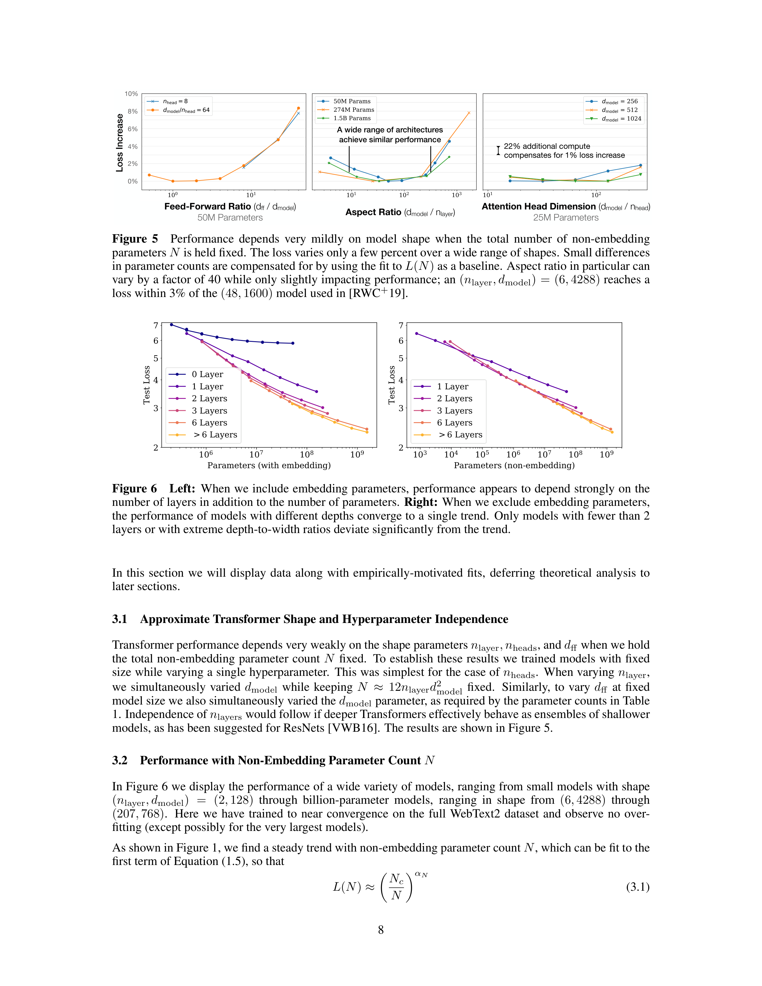
Figure
5
Performance
depends
very
mildly
on
model
shape
when
the
total
number
of
non-embedding
parameters
N
is held fixed.
The loss varies only a few percent over a wide range of shapes.
Small differences
in parameter counts are compensated for by using the fit to
L
(
N
)
as a baseline.
Aspect ratio in particular can
vary by a factor of 40 while only slightly impacting performance; an
(
n
layer
, d
model
)
=
(6
,
4288)
reaches a
loss within 3% of the
(48
,
1600)
model used in [RWC
+
19].
10
6
10
7
10
8
10
9
Parameters (with embedding)
2
3
4
5
6
7
Test Loss
0 Layer
1 Layer
2 Layers
3 Layers
6 Layers
>
6 Layers
10
3
10
4
10
5
10
6
10
7
10
8
10
9
Parameters (non-embedding)
2
3
4
5
6
7
Test Loss
1 Layer
2 Layers
3 Layers
6 Layers
>
6 Layers
Figure
6
Left:
When
we
include
embedding
parameters,
performance
appears
to
depend
strongly
on
the
number of layers in addition to the number of parameters.
Right:
When we exclude embedding parameters,
the performance of models with different depths converge to a single trend.
Only models with fewer than 2
layers or with extreme depth-to-width ratios deviate significantly from the trend.
In
this
section
we
will
display
data
along
with
empirically-motivated
fits,
deferring
theoretical
analysis
to
later sections.
3.1
Approximate Transformer Shape and Hyperparameter Independence
Transformer performance depends very weakly on the shape parameters
n
layer
, n
heads
, and
d
ff
when we hold
the
total
non-embedding
parameter
count
N
fixed.
To
establish
these
results
we
trained
models
with
fixed
size while varying a single hyperparameter.
This was simplest for the case of
n
heads
.
When varying
n
layer
,
we
simultaneously
varied
d
model
while
keeping
N
≈
12
n
layer
d
2
model
fixed.
Similarly,
to
vary
d
ff
at
fixed
model size we also simultaneously varied the
d
model
parameter, as required by the parameter counts in Table
1.
Independence of
n
layers
would follow if deeper Transformers effectively behave as ensembles of shallower
models, as has been suggested for ResNets [VWB16].
The results are shown in Figure 5.
3.2
Performance with Non-Embedding Parameter Count
N
In Figure 6 we display the performance of a wide variety of models, ranging from small models with shape
(
n
layer
, d
model
)
=
(2
,
128)
through
billion-parameter
models,
ranging
in
shape
from
(6
,
4288)
through
(207
,
768)
.
Here
we
have
trained
to
near
convergence
on
the
full
WebText2
dataset
and
observe
no
over-
fitting (except possibly for the very largest models).
As shown in Figure 1, we find a steady trend with non-embedding parameter count
N
, which can be fit to the
first term of Equation (1.5), so that
L
(
N
)
≈
N
c
N
α
N
(3.1)
8
LSTM
plateaus after <100 tokens
Transformer
improves through the whole context
2M
200M
3M
300M
5
4
3
2
6
Token Index in Context
10
3
10
2
10
1
Transformers asymptotically outperform LSTMs
due to improved use of long contexts
3.6
4.2
3.0
2.4
4.8
5.4
10
5
10
8
10
6
10
7
10
9
Parameters
(non-embedding)
Transformers
LSTMs
1 Layer
2 Layers
4 Layers
Test Loss
Per-token
Test Loss
Parameters:
400K
400K
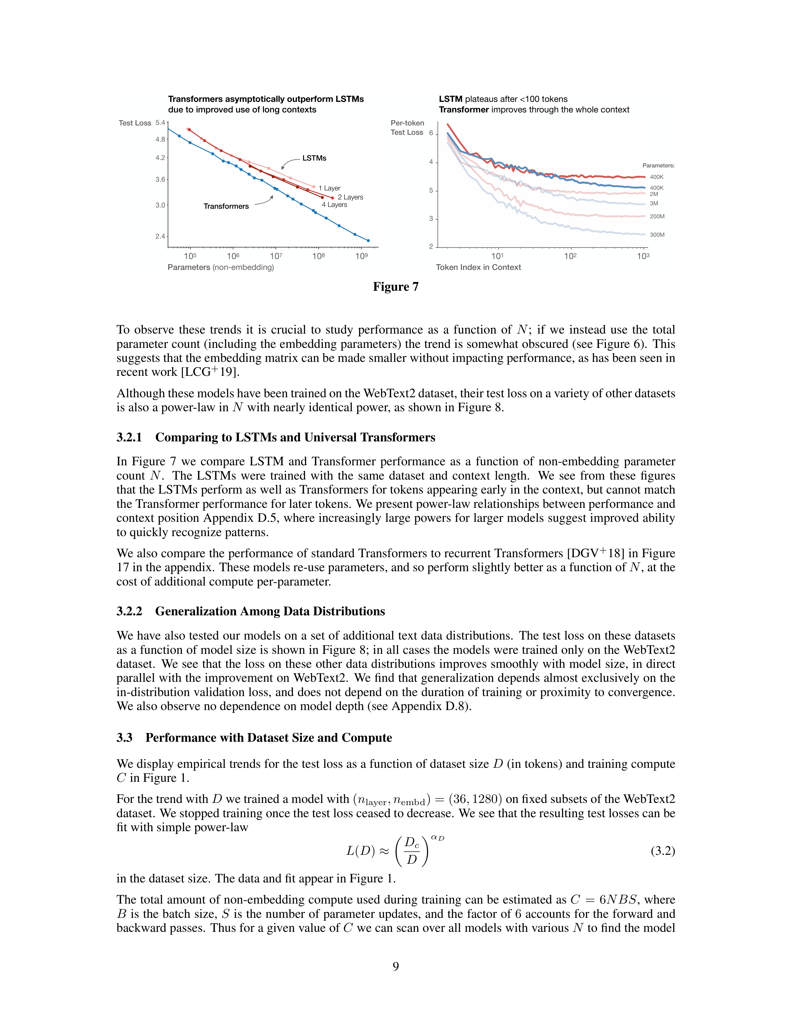
Figure 7
To
observe
these
trends
it
is
crucial
to
study
performance
as
a
function
of
N
;
if
we
instead
use
the
total
parameter count (including the embedding parameters) the trend is somewhat obscured (see Figure 6).
This
suggests that the embedding matrix can be made smaller without impacting performance, as has been seen in
recent work [LCG
+
19].
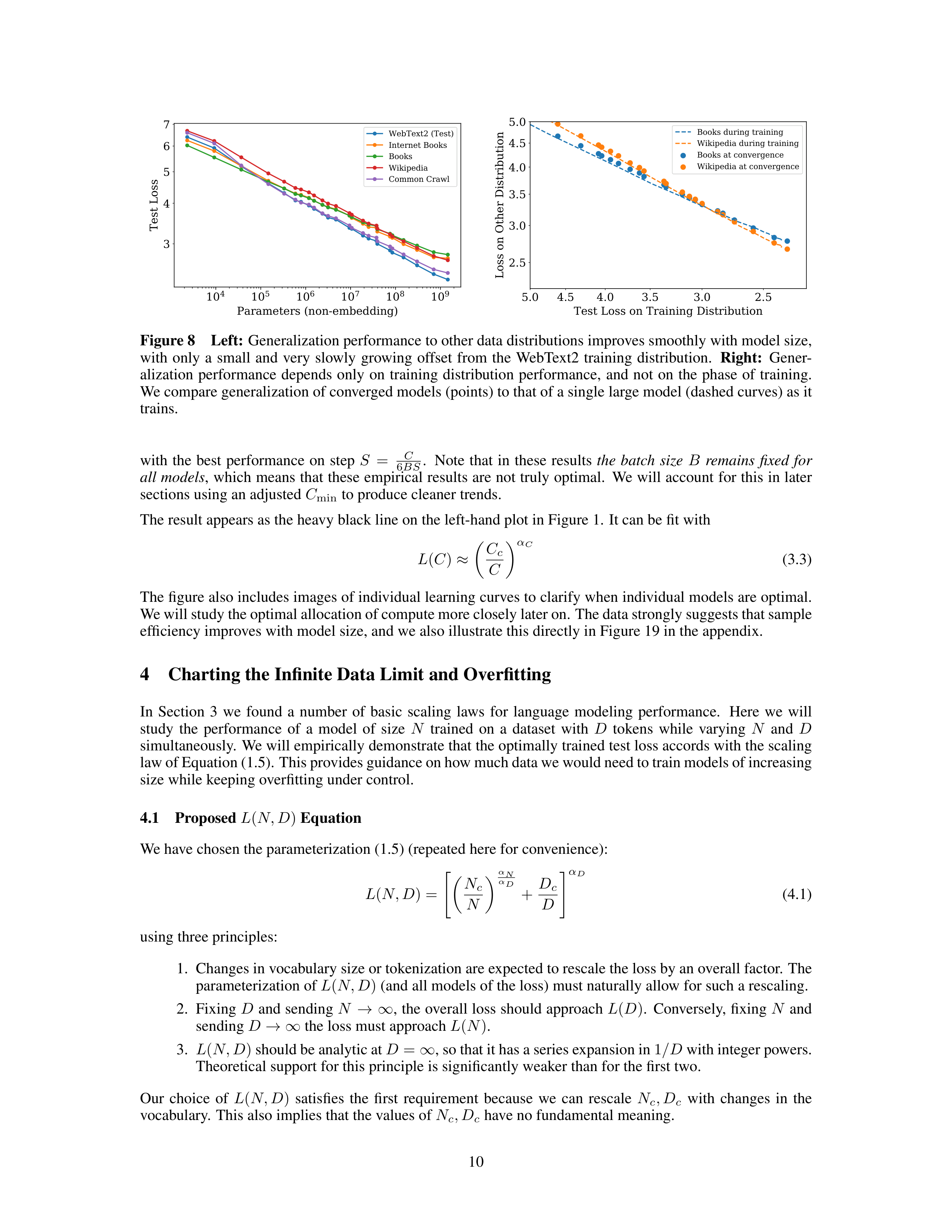
Although these models have been trained on the WebText2 dataset, their test loss on a variety of other datasets
is also a power-law in
N
with nearly identical power, as shown in Figure 8.
3.2.1
Comparing to LSTMs and Universal Transformers
In
Figure
7
we
compare
LSTM
and
Transformer
performance
as
a
function
of
non-embedding
parameter
count
N
.
The
LSTMs
were
trained
with
the
same
dataset
and
context
length.
We
see
from
these
figures
that the LSTMs perform as well as Transformers for tokens appearing early in the context, but cannot match
the Transformer performance for later tokens.
We present power-law relationships between performance and
context position Appendix D.5, where increasingly large powers for larger models suggest improved ability
to quickly recognize patterns.
We also compare the performance of standard Transformers to recurrent Transformers [DGV
+
18] in Figure
17 in the appendix.
These models re-use parameters, and so perform slightly better as a function of
N
, at the
cost of additional compute per-parameter.
3.2.2
Generalization Among Data Distributions
We have also tested our models on a set of additional text data distributions.
The test loss on these datasets
as a function of model size is shown in Figure 8; in all cases the models were trained only on the WebText2
dataset.
We see that the loss on these other data distributions improves smoothly with model size,
in direct
parallel with the improvement on WebText2.
We find that generalization depends almost exclusively on the
in-distribution validation loss, and does not depend on the duration of training or proximity to convergence.
We also observe no dependence on model depth (see Appendix D.8).
3.3
Performance with Dataset Size and Compute
We display empirical trends for the test loss as a function of dataset size
D
(in tokens) and training compute
C
in Figure 1.
For the trend with
D
we trained a model with
(
n
layer
, n
embd
) = (36
,
1280)
on fixed subsets of the WebText2
dataset.
We stopped training once the test loss ceased to decrease.
We see that the resulting test losses can be
fit with simple power-law
L
(
D
)
≈
D
c
D
α
D
(3.2)
in the dataset size.
The data and fit appear in Figure 1.
The total amount of non-embedding compute used during training can be estimated as
C
=
6
NBS
, where
B
is the batch size,
S
is the number of parameter updates,
and the factor of
6
accounts for the forward and
backward passes.
Thus for a given value of
C
we can scan over all models with various
N
to find the model
9
10
4
10
5
10
6
10
7
10
8
10
9
Parameters (non-embedding)
3
4
5
6
7
Test Loss
WebText2 (Test)
Internet Books
Books
Wikipedia
Common Crawl
2.5
3.0
3.5
4.0
4.5
5.0
Test Loss on Training Distribution
2.5
3.0
3.5
4.0
4.5
5.0
Loss on Other Distribution
Books during training
Wikipedia during training
Books at convergence
Wikipedia at convergence
Figure 8
Left:
Generalization performance to other data distributions improves smoothly with model size,
with
only
a
small
and
very
slowly
growing
offset
from
the
WebText2
training
distribution.
Right:
Gener-
alization
performance
depends
only
on
training
distribution
performance,
and
not
on
the
phase
of
training.
We compare generalization of converged models (points) to that of a single large model (dashed curves) as it
trains.
with
the
best
performance
on
step
S
=
C
6
BS
.
Note
that
in
these
results
the
batch
size
B
remains
fixed
for
all models
,
which means that these empirical results are not truly optimal.
We will account for this in later
sections using an adjusted
C
min
to produce cleaner trends.
The result appears as the heavy black line on the left-hand plot in Figure 1.
It can be fit with
L
(
C
)
≈
C
c
C
α
C
(3.3)
The figure also includes images of individual learning curves to clarify when individual models are optimal.
We will study the optimal allocation of compute more closely later on. The data strongly suggests that sample
efficiency improves with model size, and we also illustrate this directly in Figure 19 in the appendix.
4
Charting the Infinite Data Limit and Overfitting
In
Section
3
we
found
a
number
of
basic
scaling
laws
for
language
modeling
performance.
Here
we
will
study
the
performance
of
a
model
of
size
N
trained
on
a
dataset
with
D
tokens
while
varying
N
and
D
simultaneously.
We will empirically demonstrate that the optimally trained test loss accords with the scaling
law of Equation (1.5). This provides guidance on how much data we would need to train models of increasing
size while keeping overfitting under control.
4.1
Proposed
L
(
N, D
)
Equation
We have chosen the parameterization (1.5) (repeated here for convenience):
L
(
N, D
) =
"
N
c
N
α
N
αD
+
D
c
D
#
α
D
(4.1)
using three principles:
1.
Changes in vocabulary size or tokenization are expected to rescale the loss by an overall factor.
The
parameterization of
L
(
N, D
)
(and all models of the loss) must naturally allow for such a rescaling.
2.
Fixing
D
and sending
N
→∞
, the overall loss should approach
L
(
D
)
.
Conversely, fixing
N
and
sending
D
→∞
the loss must approach
L
(
N
)
.
3.
L
(
N, D
)
should be analytic at
D
=
∞
, so that it has a series expansion in
1
/D
with integer powers.
Theoretical support for this principle is significantly weaker than for the first two.
Our
choice
of
L
(
N, D
)
satisfies
the
first
requirement
because
we
can
rescale
N
c
, D
c
with
changes
in
the
vocabulary.
This also implies that the values of
N
c
, D
c
have no fundamental meaning.
10
10
6
10
7
10
8
10
9
Params (non-embed)
2.5
3.0
3.5
4.0
4.5
Test Loss
Data Size Bottleneck
Data Size
21M
43M
86M
172M
344M
688M
1.4B
22.0B
10
4
10
3
10
2
10
1
N
N
/
D
/
D
0.0
0.1
0.2
0.3
0.4
0.5
L
/
L
(
D
=
)
1
Overfitting
Data Size
21M
43M
86M
172M
344M
688M
1.4B
22.0B
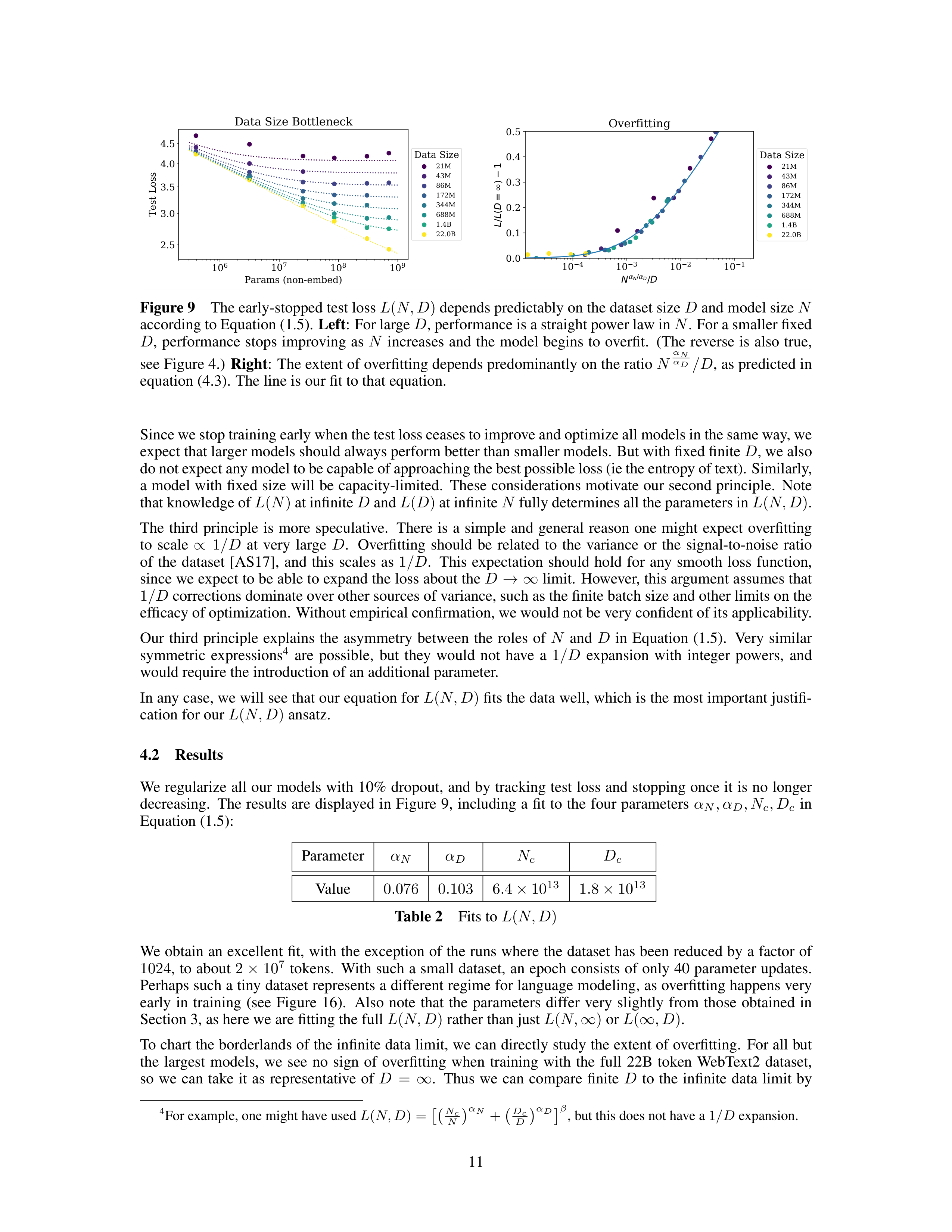
Figure 9
The early-stopped test loss
L
(
N, D
)
depends predictably on the dataset size
D
and model size
N
according to Equation (1.5).
Left
:
For large
D
, performance is a straight power law in
N
.
For a smaller fixed
D
,
performance
stops
improving
as
N
increases
and
the
model
begins
to
overfit.
(The
reverse
is
also
true,
see Figure 4.)
Right
:
The extent of overfitting depends predominantly on the ratio
N
αN
αD
/D
, as predicted in
equation (4.3).
The line is our fit to that equation.
Since we stop training early when the test loss ceases to improve and optimize all models in the same way, we
expect that larger models should always perform better than smaller models.
But with fixed finite
D
, we also
do not expect any model to be capable of approaching the best possible loss (ie the entropy of text). Similarly,
a model with fixed size will be capacity-limited.
These considerations motivate our second principle.
Note
that knowledge of
L
(
N
)
at infinite
D
and
L
(
D
)
at infinite
N
fully determines all the parameters in
L
(
N, D
)
.
The
third
principle
is
more
speculative.
There
is
a
simple
and
general
reason
one
might
expect
overfitting
to
scale
∝
1
/D
at
very
large
D
.
Overfitting
should
be
related
to
the
variance
or
the
signal-to-noise
ratio
of
the
dataset
[AS17],
and
this
scales
as
1
/D
.
This
expectation
should
hold
for
any
smooth
loss
function,
since we expect to be able to expand the loss about the
D
→∞
limit.
However, this argument assumes that
1
/D
corrections dominate over other sources of variance, such as the finite batch size and other limits on the
efficacy of optimization.
Without empirical confirmation, we would not be very confident of its applicability.
Our
third
principle
explains
the
asymmetry
between
the
roles
of
N
and
D
in
Equation
(1.5).
Very
similar
symmetric
expressions
4
are
possible,
but
they
would
not
have
a
1
/D
expansion
with
integer
powers,
and
would require the introduction of an additional parameter.
In any case, we will see that our equation for
L
(
N, D
)
fits the data well, which is the most important justifi-
cation for our
L
(
N, D
)
ansatz.
4.2
Results
We regularize all our models with 10% dropout,
and by tracking test loss and stopping once it is no longer
decreasing.
The
results
are
displayed
in
Figure
9,
including
a
fit
to
the
four
parameters
α
N
, α
D
, N
c
, D
c
in
Equation (1.5):
Parameter
α
N
α
D
N
c
D
c
Value
0
.
076
0
.
103
6
.
4
×
10
13
1
.
8
×
10
13
Table 2
Fits to
L
(
N, D
)
We obtain an excellent fit,
with the exception of the runs where the dataset has been reduced by a factor of
1024
,
to about
2
×
10
7
tokens.
With such a small dataset,
an epoch consists of only 40 parameter updates.
Perhaps such a tiny dataset represents a different regime for language modeling, as overfitting happens very
early
in
training
(see
Figure
16).
Also
note
that
the
parameters
differ
very
slightly
from
those
obtained
in
Section 3, as here we are fitting the full
L
(
N, D
)
rather than just
L
(
N,
∞
)
or
L
(
∞
, D
)
.
To chart the borderlands of the infinite data limit, we can directly study the extent of overfitting.
For all but
the
largest
models,
we
see
no
sign
of
overfitting
when
training
with
the
full
22B
token
WebText2
dataset,
so
we
can
take
it
as
representative
of
D
=
∞
.
Thus
we
can
compare
finite
D
to
the
infinite
data
limit
by
4
For example, one might have used
L
(
N, D
) =
N
c
N
α
N
+
D
c
D
α
D
β
, but this does not have a
1
/D
expansion.
11
10
1
3 × 10
0
4 × 10
0
6 × 10
0
WebText2 Train Loss
10
3
10
4
10
5
10
6
Critical Batch Size (Tokens)
Critical Batch Size vs. Performance
Empirical
B
crit
,
N
=
3M
Empirical
B
crit
,
N
=
85M
B
crit
= 2.1 × 10
8
tokens
L
4.8
Noise Scale Measurement
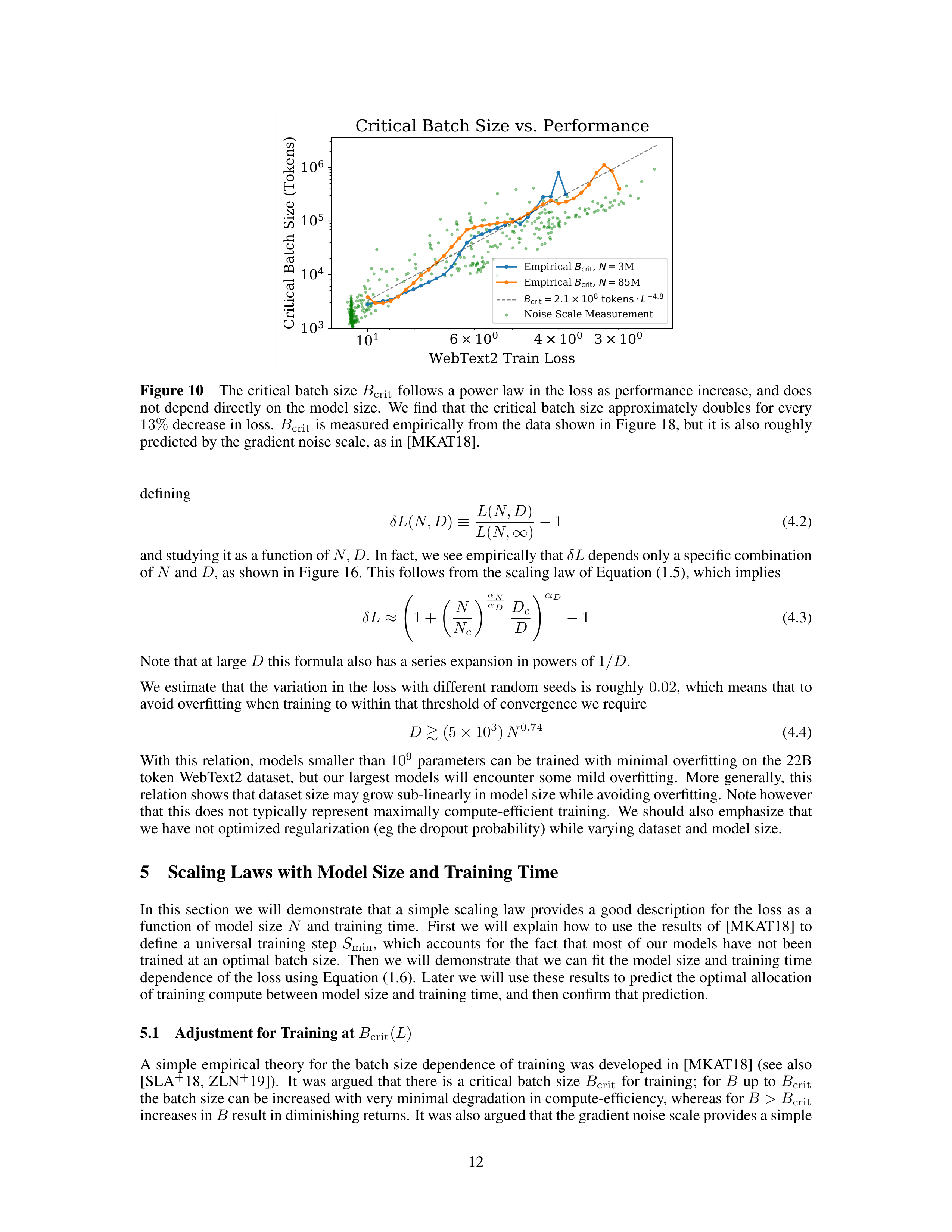
Figure 10
The critical batch size
B
crit
follows a power law in the loss as performance increase, and does
not
depend
directly
on
the
model
size.
We
find
that
the
critical
batch
size
approximately
doubles
for
every
13%
decrease in loss.
B
crit
is measured empirically from the data shown in Figure 18, but it is also roughly
predicted by the gradient noise scale, as in [MKAT18].
defining
δL
(
N, D
)
≡
L
(
N, D
)
L
(
N,
∞
)
−
1
(4.2)
and studying it as a function of
N, D
.
In fact, we see empirically that
δL
depends only a specific combination
of
N
and
D
, as shown in Figure 16.
This follows from the scaling law of Equation (1.5), which implies
δL
≈
1 +
N
N
c
α
N
αD
D
c
D
!
α
D
−
1
(4.3)
Note that at large
D
this formula also has a series expansion in powers of
1
/D
.
We estimate
that
the
variation
in
the
loss with different random
seeds
is roughly
0
.
02
,
which means that to
avoid overfitting when training to within that threshold of convergence we require
D
≳
(5
×
10
3
)
N
0
.
74
(4.4)
With
this
relation,
models
smaller
than
10
9
parameters
can
be
trained
with
minimal
overfitting
on
the
22B
token
WebText2
dataset,
but
our
largest
models
will
encounter
some
mild
overfitting.
More
generally,
this
relation shows that dataset size may grow sub-linearly in model size while avoiding overfitting. Note however
that
this
does
not
typically
represent
maximally
compute-efficient
training.
We
should
also
emphasize
that
we have not optimized regularization (eg the dropout probability) while varying dataset and model size.
5
Scaling Laws with Model Size and Training Time
In
this
section
we
will
demonstrate
that
a
simple
scaling
law
provides
a
good
description
for
the
loss
as
a
function
of
model
size
N
and
training
time.
First
we
will
explain
how
to
use
the
results
of
[MKAT18]
to
define
a
universal
training
step
S
min
,
which
accounts
for
the
fact
that
most
of
our
models
have
not
been
trained at an optimal batch size.
Then we will demonstrate that we can fit the model size and training time
dependence of the loss using Equation (1.6).
Later we will use these results to predict the optimal allocation
of training compute between model size and training time, and then confirm that prediction.
5.1
Adjustment for Training at
B
crit
(
L
)
A simple empirical theory for the batch size dependence of training was developed in [MKAT18] (see also
[SLA
+
18,
ZLN
+
19]).
It
was
argued
that
there
is
a
critical
batch
size
B
crit
for
training;
for
B
up
to
B
crit
the batch size can be increased with very minimal degradation in compute-efficiency, whereas for
B
> B
crit
increases in
B
result in diminishing returns.
It was also argued that the gradient noise scale provides a simple
12
prediction for
B
crit
, and that neither depends directly on model size except through the value of the loss that
has
been
attained.
These
results
can
be
used
to
predict
how
training
time
and
compute
will
vary
with
the
batch size.
To utilize both training time and compute as effectively as possible, it is best to train with a batch
size
B
≈
B
crit
.
Training at
B
≫
B
crit
minimizes the number of training steps, while
B
≪
B
crit
minimizes
the use of compute.
More specifically, it was demonstrated that for a wide variety of neural network tasks, the number of training
steps
S
and the number of data examples processed
E
=
BS
satisfy the simple relation
S
S
min
−
1
E
E
min
−
1
= 1
(5.1)
when training to any fixed value of the loss
L
.
Here
S
min
is the minimum number of steps necessary to reach
L
, while
E
min
is the minimum number of data examples that must be processed.
We
demonstrate
the
relation
(5.1)
for
Transformers
in
Figure
18
in
the
appendix.
This
relation
defines
the
critical batch size
B
crit
(
L
)
≡
E
min
S
min
(5.2)
which is a function of the target value of the loss.
Training at the critical batch size makes a roughly optimal
time/compute tradeoff, requiring
2
S
min
training steps and processing
E
= 2
E
min
data examples.
In Figure 10 we have plotted the critical batch size and gradient noise scale
5
as a function of training loss for
two different models.
We see that
B
crit
(
L
)
is independent of model size, and only depends on the loss
L
.
So
the predictions of [MKAT18] continue to hold for Transformer language models.
The critical batch size can
be fit with a power-law in the loss
B
crit
(
L
)
≈
B
∗
L
1
/α
B
(5.3)
where
B
∗
≈
2
×
10
8
and
α
B
≈
0
.
21
.
We have chosen this parameterization for
B
crit
(
L
)
because as the loss approaches its minimum value
L
min
,
the
gradient
noise
scale
is
expected
to
diverge,
and
we
expect
B
crit
to
track
this
noise
scale.
We
do
not
know
L
min
, as we see no sign that our models are approaching it, but
L
min
>
0
since the entropy of natural
language is non-zero.
Since apparently
L
min
is much smaller than the values of
L
we have achieved, we used
a parameterization where
B
crit
diverges as
L
→
0
.
We will use
B
crit
(
L
)
to estimate the relation between the number of training steps
S
while training at batch
size
B
= 2
19
tokens and the number of training steps while training at
B
≫
B
crit
.
This is simply
S
min
(
S
)
≡
S
1 +
B
crit
(
L
)
/B
(
minimum steps, at
B
≫
B
crit
)
(5.4)
for any given target value
L
for the loss.
This also defines a critical value of the compute needed to train to
L
with a model of size
N
if we were to train at
B
≪
B
crit
(
L
)
.
This is
C
min
(
C
)
≡
C
1 +
B/B
crit
(
L
)
(
minimum compute, at
B
≪
B
crit
)
(5.5)
where
C
= 6
NBS
estimates the (non-embedding) compute used at batch size
B
.
5.2
Results for
L
(
N, S
min
)
and Performance with Model Size and Compute
Now we will use
S
min
defined in Equation (5.4) to obtain a simple and universal fit for the dependence of the
loss on model size and training time in the infinite data limit.
We will fit the stable, Adam-optimized training
runs using Equation (1.6), repeated here for convenience:
L
(
N, S
min
) =
N
c
N
α
N
+
S
c
S
min
α
S
(5.6)
for the loss.
We include all training steps after the warmup period of the learning rate schedule, and find a fit
to the data with the parameters:
5
Although
the
critical
batch
size
roughly
matches
the
gradient
noise
scale,
we
are
using
a
direct
measurements
of
B
crit
from Figures 18 and 10 for all our later analyses.
13


10
4
10
6
10
8
Parameters (non-embedding)
2
3
4
5
6
7
8
Test Loss
Performance vs Compute Budget
10
5
10
4
10
3
10
2
10
1
10
0
PF-dayss
10
6
10
7
10
8
10
9
Parameters (non-embedding)
2.4
3.0
3.6
4.2
4.8
5.4
Test Loss
Performance vs Steps
10
4
10
5
Steps
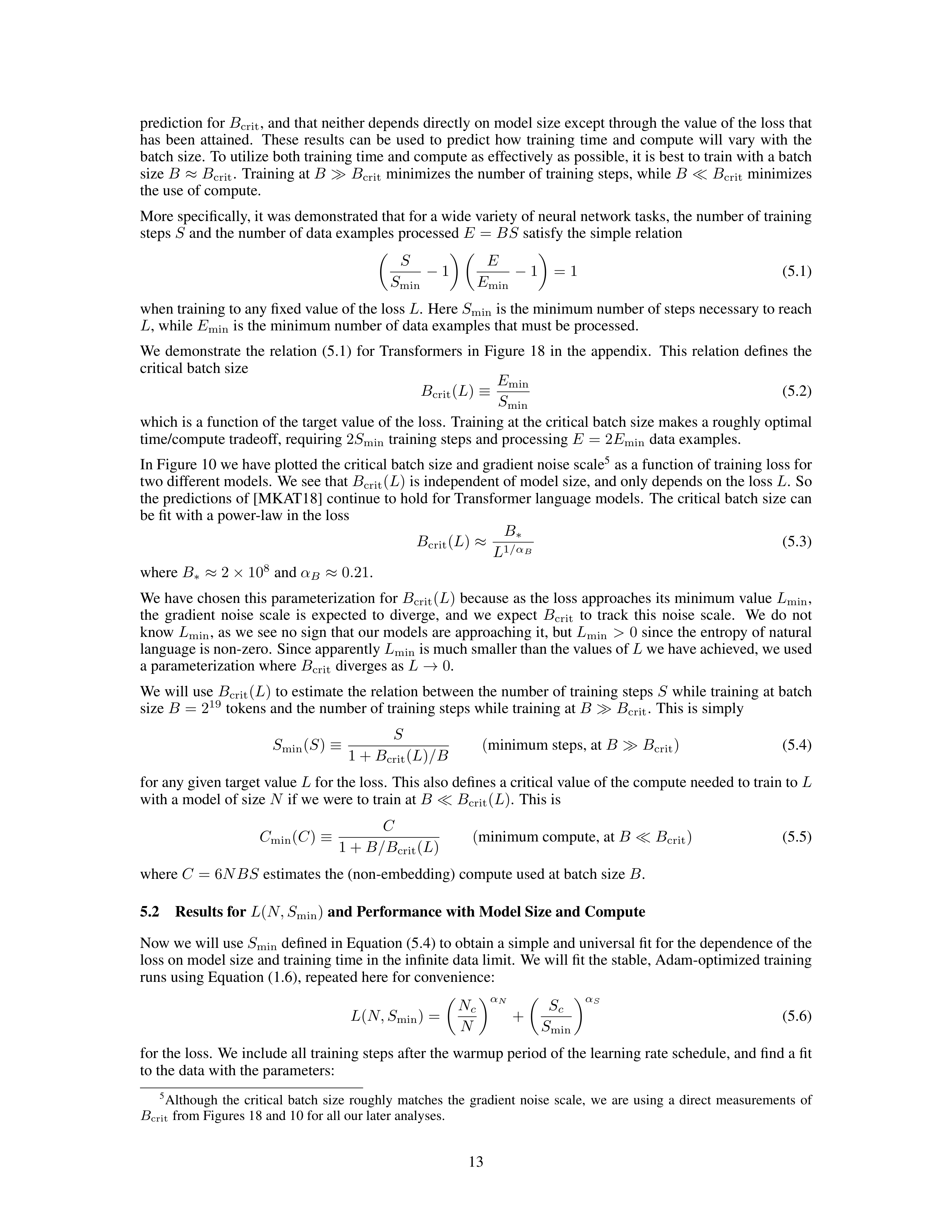
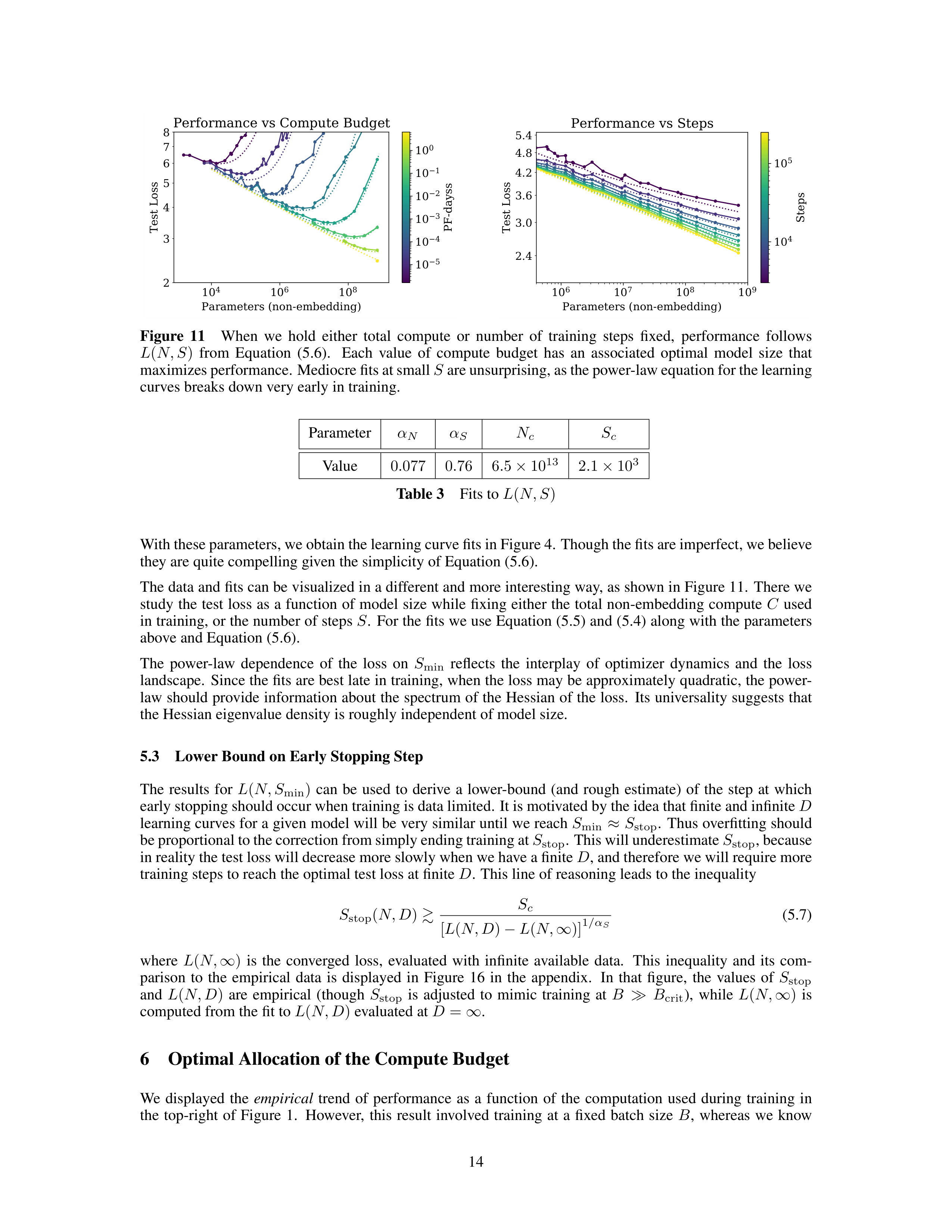
Figure
11
When
we
hold
either
total
compute
or
number
of
training
steps
fixed,
performance
follows
L
(
N, S
)
from
Equation
(5.6).
Each
value
of
compute
budget
has
an
associated
optimal
model
size
that
maximizes performance. Mediocre fits at small
S
are unsurprising, as the power-law equation for the learning
curves breaks down very early in training.
Parameter
α
N
α
S
N
c
S
c
Value
0
.
077
0
.
76
6
.
5
×
10
13
2
.
1
×
10
3
Table 3
Fits to
L
(
N, S
)
With these parameters, we obtain the learning curve fits in Figure 4.
Though the fits are imperfect, we believe
they are quite compelling given the simplicity of Equation (5.6).
The data and fits can be visualized in a different and more interesting way, as shown in Figure 11.
There we
study the test loss as a function of model size while fixing either the total non-embedding compute
C
used
in training, or the number of steps
S
.
For the fits we use Equation (5.5) and (5.4) along with the parameters
above and Equation (5.6).
The
power-law
dependence
of
the
loss
on
S
min
reflects
the
interplay
of
optimizer
dynamics
and
the
loss
landscape.
Since the fits are best late in training, when the loss may be approximately quadratic, the power-
law should provide information about the spectrum of the Hessian of the loss.
Its universality suggests that
the Hessian eigenvalue density is roughly independent of model size.
5.3
Lower Bound on Early Stopping Step
The
results
for
L
(
N, S
min
)
can
be
used
to
derive
a
lower-bound
(and
rough
estimate)
of
the
step
at
which
early stopping should occur when training is data limited.
It is motivated by the idea that finite and infinite
D
learning curves for a given model will be very similar until we reach
S
min
≈
S
stop
.
Thus overfitting should
be proportional to the correction from simply ending training at
S
stop
. This will underestimate
S
stop
, because
in reality the test loss will decrease more slowly when we have a finite
D
, and therefore we will require more
training steps to reach the optimal test loss at finite
D
.
This line of reasoning leads to the inequality
S
stop
(
N, D
)
≳
S
c
[
L
(
N, D
)
−
L
(
N,
∞
)]
1
/α
S
(5.7)
where
L
(
N,
∞
)
is
the
converged
loss,
evaluated
with
infinite
available
data.
This
inequality
and
its
com-
parison
to
the
empirical
data
is
displayed
in
Figure
16
in
the
appendix.
In
that
figure,
the
values
of
S
stop
and
L
(
N, D
)
are
empirical
(though
S
stop
is
adjusted
to
mimic
training
at
B
≫
B
crit
),
while
L
(
N,
∞
)
is
computed from the fit to
L
(
N, D
)
evaluated at
D
=
∞
.
6
Optimal Allocation of the Compute Budget
We
displayed
the
empirical
trend
of
performance
as
a
function
of
the
computation
used
during
training
in
the
top-right
of
Figure
1.
However,
this
result
involved
training
at
a
fixed
batch
size
B
,
whereas
we
know
14
Models between 0.6x and 2.2x the
optimal size can be trained with a
20% larger compute budget
Smaller models require
more steps to train, while
larger models require fewer
Our framework does not
capture early training dynamics
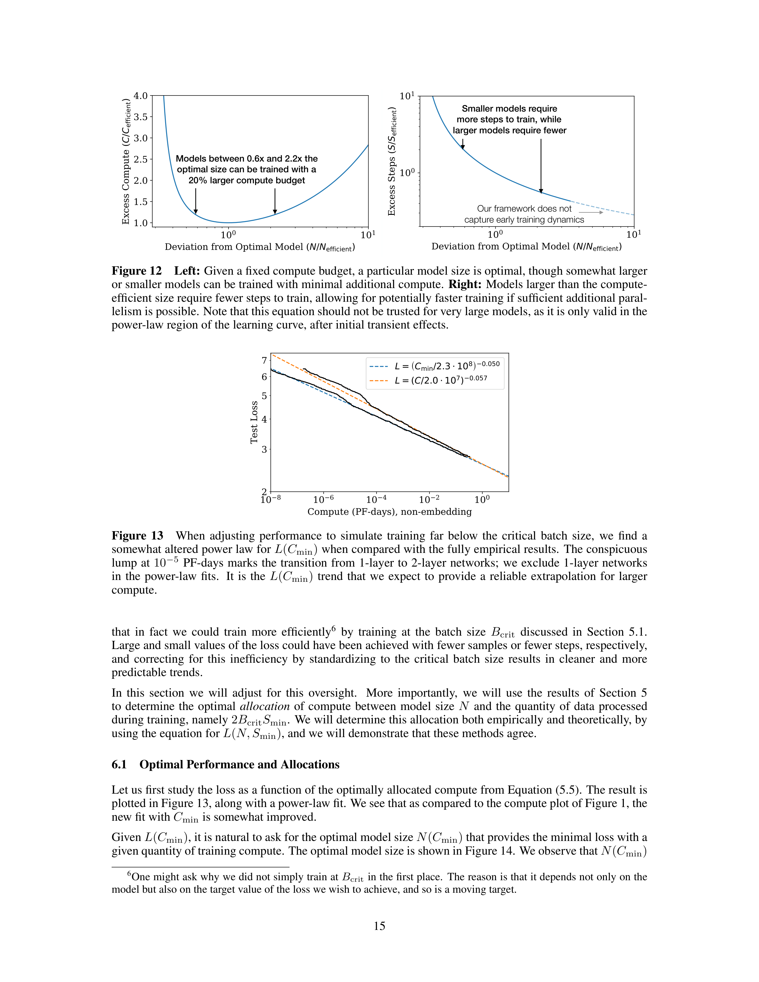
Figure 12
Left:
Given a fixed compute budget, a particular model size is optimal, though somewhat larger
or smaller models can be trained with minimal additional compute.
Right:
Models larger than the compute-
efficient size require fewer steps to train, allowing for potentially faster training if sufficient additional paral-
lelism is possible.
Note that this equation should not be trusted for very large models, as it is only valid in the
power-law region of the learning curve, after initial transient effects.
10
8
10
6
10
4
10
2
10
0
Compute (PF-days), non-embedding
2
3
4
5
6
7
Test Loss
L
=
(
C
min
/2.3
10
8
)
0.050
L
= (
C
/2.0
10
7
)
0.057
Figure
13
When
adjusting
performance
to
simulate
training
far
below
the
critical
batch
size,
we
find
a
somewhat altered power law for
L
(
C
min
)
when compared with the fully empirical results.
The conspicuous
lump
at
10
−
5
PF-days
marks
the
transition
from
1-layer
to
2-layer
networks;
we
exclude
1-layer
networks
in
the
power-law
fits.
It
is
the
L
(
C
min
)
trend
that
we
expect
to
provide
a
reliable
extrapolation
for
larger
compute.
that
in
fact
we
could
train
more
efficiently
6
by
training
at
the
batch
size
B
crit
discussed
in
Section
5.1.
Large and small values of the loss could have been achieved with fewer samples or fewer steps, respectively,
and
correcting
for
this
inefficiency
by
standardizing
to
the
critical
batch
size
results
in
cleaner
and
more
predictable trends.
In
this
section
we
will
adjust
for
this
oversight.
More
importantly,
we
will
use
the
results
of
Section
5
to
determine
the
optimal
allocation
of
compute
between
model
size
N
and
the
quantity
of
data
processed
during training, namely
2
B
crit
S
min
.
We will determine this allocation both empirically and theoretically, by
using the equation for
L
(
N, S
min
)
, and we will demonstrate that these methods agree.
6.1
Optimal Performance and Allocations
Let us first study the loss as a function of the optimally allocated compute from Equation (5.5).
The result is
plotted in Figure 13, along with a power-law fit.
We see that as compared to the compute plot of Figure 1, the
new fit with
C
min
is somewhat improved.
Given
L
(
C
min
)
, it is natural to ask for the optimal model size
N
(
C
min
)
that provides the minimal loss with a
given quantity of training compute.
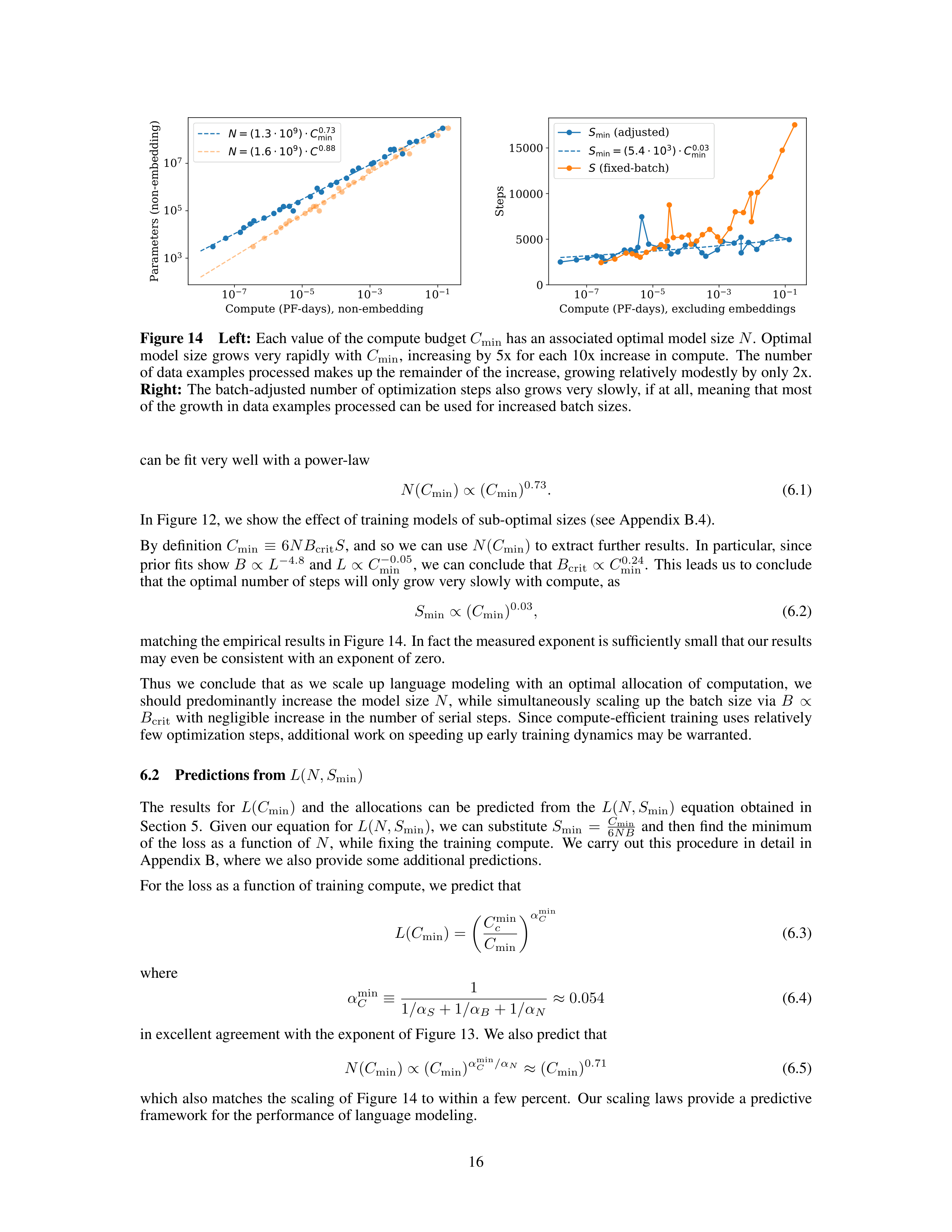
The optimal model size is shown in Figure 14.
We observe that
N
(
C
min
)
6
One might ask why we did not simply train at
B
crit
in the first place.
The reason is that it depends not only on the
model but also on the target value of the loss we wish to achieve, and so is a moving target.
15
10
7
10
5
10
3
10
1
Compute (PF-days), non-embedding
10
3
10
5
10
7
Parameters (non-embedding)
N
= (1.3
10
9
)
C
0.73
min
N
= (1.6
10
9
)
C
0.88
10
7
10
5
10
3
10
1
Compute (PF-days), excluding embeddings
0
5000
10000
15000
Steps
S
min
(adjusted)
S
min
= (5.4
10
3
)
C
0.03
min
S
(fixed-batch)
Figure 14
Left:
Each value of the compute budget
C
min
has an associated optimal model size
N
.
Optimal
model size grows very rapidly with
C
min
,
increasing by 5x for each 10x increase in compute.
The number
of data examples processed makes up the remainder of the increase, growing relatively modestly by only 2x.
Right:
The batch-adjusted number of optimization steps also grows very slowly, if at all, meaning that most
of the growth in data examples processed can be used for increased batch sizes.
can be fit very well with a power-law
N
(
C
min
)
∝
(
C
min
)
0
.
73
.
(6.1)
In Figure 12, we show the effect of training models of sub-optimal sizes (see Appendix B.4).
By definition
C
min
≡
6
NB
crit
S
, and so we can use
N
(
C
min
)
to extract further results.
In particular, since
prior fits show
B
∝
L
−
4
.
8
and
L
∝
C
−
0
.
05
min
, we can conclude that
B
crit
∝
C
0
.
24
min
.
This leads us to conclude
that the optimal number of steps will only grow very slowly with compute, as
S
min
∝
(
C
min
)
0
.
03
,
(6.2)
matching the empirical results in Figure 14. In fact the measured exponent is sufficiently small that our results
may even be consistent with an exponent of zero.
Thus
we
conclude
that
as
we
scale
up
language
modeling
with
an
optimal
allocation
of
computation,
we
should
predominantly
increase
the
model
size
N
,
while
simultaneously
scaling
up
the
batch
size
via
B
∝
B
crit
with negligible increase in the number of serial steps.
Since compute-efficient training uses relatively
few optimization steps, additional work on speeding up early training dynamics may be warranted.
6.2
Predictions from
L
(
N, S
min
)
The
results
for
L
(
C
min
)
and
the
allocations
can
be
predicted
from
the
L
(
N, S
min
)
equation
obtained
in
Section 5.
Given our equation for
L
(
N, S
min
)
,
we can substitute
S
min
=
C
min
6
NB
and then find the minimum
of
the
loss
as
a
function
of
N
,
while
fixing
the
training
compute.
We
carry
out
this
procedure
in
detail
in
Appendix B, where we also provide some additional predictions.
For the loss as a function of training compute, we predict that
L
(
C
min
) =
C
min
c
C
min
α
min
C
(6.3)
where
α
min
C
≡
1
1
/α
S
+ 1
/α
B
+ 1
/α
N
≈
0
.
054
(6.4)
in excellent agreement with the exponent of Figure 13.
We also predict that
N
(
C
min
)
∝
(
C
min
)
α
min
C
/α
N
≈
(
C
min
)
0
.
71
(6.5)
which also matches the scaling of Figure 14 to within a few percent.
Our scaling laws provide a predictive
framework for the performance of language modeling.
16
The intersection point is sensitive to
the precise power-law parameters
Figure 15
Far beyond the model sizes we study empirically, we find a contradiction between our equations
for
L
(
C
min
)
and
L
(
D
)
due to the slow growth of data needed for compute-efficient training.
The intersection
marks the point before which we expect our predictions to break down.
The location of this point is highly
sensitive to the precise exponents from our power-law fits.
6.3
Contradictions and a Conjecture
We observe no signs of deviation from straight power-law trends at large values of compute, data, or model
size.
Our trends must eventually level off, though, since natural language has non-zero entropy.
Indeed, the trends for compute-efficient training described in this section already contain an apparent contra-
diction.
At scales several orders of magnitude above those documented here,
the performance predicted by
the
L
(
C
min
)
scaling law decreases below what should be possible given the slow growth in training data with
compute.
This
implies
that
our
scaling
laws
must
break
down
before
this
point,
but
we
conjecture
that
the
intersection point has a deeper meaning:
it provides an estimate of the point at which Transformer language
models reach maximal performance.
Since
the
amount
of
data
used
by
compute-efficient
training
grows
slowly
with
the
compute
budget,
the
performance predicted by
L
(
C
min
)
eventually hits a lower bound set by the
L
(
D
)
power law (see Figure 15).
Let us work this out in more detail.
To keep overfitting under control, the results of Section 4 imply that we should scale the dataset size as
D
∝
N
0
.
74
∝
C
0
.
54
min
(6.6)
where we have used the compute-efficient
N
(
C
min
)
from Figure 14.
Let
us
compare
this
to
the
data
requirements
of
compute-efficient
training.
If
we
train
at
the
critical
batch
size (i.e.
C
= 2
C
min
) and never re-use data during training, we find that data usage grows with compute as
D
(
C
min
) =
2
C
min
6
N
(
C
min
)
≈
4
×
10
10
tokens
(
C
min
/
PF
-
Day)
0
.
26
(6.7)
This is the maximum rate at which the dataset size can productively grow with compute, since it means that
we are only training for a single epoch.
But it grows the dataset much more slowly than in Equation (6.6).
It appears to imply that compute-efficient training will eventually run into a problem with overfitting, even if
the training process never re-uses any data!
According
to
Figure
1,
we
expect
that
when
we
are
bottlenecked
by
the
dataset
size
(ie
by
overfitting),
the
loss should scale as
L
(
D
)
∝
D
−
0
.
095
. This implies that the loss would scale with compute as
L
(
D
(
C
min
))
∝
C
−
0
.
03
min
once we are data-limited.
Once again, we have a contradiction, as this will eventually intersect with
our prediction for
L
(
C
min
)
from Figure 13, where we found a scaling
L
(
C
min
)
∝
C
−
0
.
050
min
.
The intersection point of
L
(
D
(
C
min
))
and
L
(
C
min
)
occurs at
C
∗
∼
10
4
PF
-
Days
N
∗
∼
10
12
parameters
,
D
∗
∼
10
12
tokens
,
L
∗
∼
1
.
7
nats/token
(6.8)
though
the
numerical
values
are
highly
uncertain,
varying
by
an
order
or
magnitude
in
either
direction
de-
pending on the precise values of the exponents from the power-law fits.
The most obvious interpretation is
that
our
scaling
laws
break
down
at
or
before
we
reach
this
point,
which
is
still
many
orders
of
magnitude
away in both compute and model size.
17
One might also conjecture that this intersection point has a deeper meaning.
If we cannot increase the model
size
beyond
N
∗
without
qualitatively
different
data
requirements,
perhaps
this
means
that
once
we
reach
C
∗
min
and
N
∗
,
we
have
extracted
all
of
the
reliable
information
available
in
natural
language
data.
In
this
interpretation,
L
∗
would
provide
a
rough
estimate
for
the
entropy-per-token
7
of
natural
language.
In
this
scenario, we would expect the loss trend to level off at or before
L
∗
.
We
can
guess
at
the
functional
form
of
L
(
C
min
)
as
it
levels
off
by
considering
a
version
of
our
training
dataset
with
added
noise.
For
example,
we
could
append
a
random
string
of
tokens
to
each
context
shown
to
the
model
to
artificially
boost
the
loss
by
a
constant
additive
factor.
Then,
the
distance
from
the
noise
floor
L
−
L
noise
would be a more meaningful performance metric, with even a small decrease in this distance
potentially representing a significant boost in qualitative performance.
Since the artificial noise would affect
all of our trends equally, the critical point of 6.8 would not change (aside from the absolute value of
L
∗
), and
may be meaningful even if it occurs after the leveling off.
7
Related Work
Power laws can arise from a wide variety of sources [THK18].
Power-law scalings with model and dataset
size in density estimation [Was06] and in random forest models [Bia12] may be connected with our results.
These
models
suggest
that
power-law
exponents
may
have
a
very
rough
interpretation
as
the
inverse
of
the
number of relevant features in the data.
Some
early
[BB01,
Goo01]
work
found
power-law
scalings
between
performance
and
dataset
size.
More
recent
work
[HNA
+
17,
HAD19]
also
investigated
scaling
between
model
size
and
data
size;
their
work
is
perhaps
the
closest
to
ours
in
the
literature
8
.
Note,
however,
that
[HNA
+
17]
found
super-linear
scaling
of
dataset
size
with
model
size,
whereas
we
find
a
sub-linear
scaling.
There
are
some
parallels
between
our
findings on optimal allocation of compute and [Kom19], including power-law learning curves.
EfficientNets
[TL19] also appear to obey an approximate power-law relation between accuracy and model size. Very recent
work [RRBS19b] studies scaling with both dataset size and model size for a variety of datasets,
and fits an
ansatz similar to ours.
EfficientNet [TL19] advocates scaling depth and width exponentially (with different coefficients) for optimal
performance of image models, resulting in a power-law scaling of width as a function of depth.
We find that
for language models this power should be roughly one when scaling up (as width/depth should remain fixed).
But more importantly, we find that the precise architectural hyperparameters are unimportant compared to the
overall scale of the language model.
In [VWB16] it was argued that deep models can function as ensembles
of shallower models, which could potentially explain this finding.
Earlier work [ZK16] has compared width
and depth, and found that wide ResNets can outperform deep ResNets on image classification.
Some studies
fix
computation
per
data
example,
which
tends
to
scale
in
proportion
to
the
number
of
model
parameters,
whereas we investigate scaling with both model size and the quantity of training computation.
Various works [AS17, BHMM18] have investigated generalization in highly overparameterized models, find-
ing a “jamming transition” [GJS
+
19] when the model size reaches the dataset size (this may require training
many
orders
of
magnitude
beyond
typical
practice,
and
in
particular
does
not
use
early
stopping).
We
do
not
observe
such
a
transition,
and
find
that
the
necessary
training
data
scales
sublinearly
in
the
model
size.
Expansions in the model size, particularly at large width [JGH18, LXS
+
19], may provide a useful framework
for thinking about some of our scaling relations.
Our results on optimization,
such as the shape of learning
curves, can likely be explained using a noisy quadratic model, which can provide quite accurate predictions
[ZLN
+
19]
in
realistic
settings.
Making
this
connection
quantitative
will
require
a
characterization
of
the
Hessian spectrum [Pap18, GKX19, GARD18].
8
Discussion
We have observed consistent scalings of language model log-likelihood loss with non-embedding parameter
count
N
,
dataset size
D
,
and optimized training computation
C
min
,
as encapsulated in Equations (1.5) and
(1.6).
Conversely, we find very weak dependence on many architectural and optimization hyperparameters.
Since scalings with
N, D, C
min
are power-laws, there are diminishing returns with increasing scale.
7
Defining words using the
wc
utility, the WebText2 dataset has
1
.
4
tokens per word and
4
.
3
characters per token.
8
After this
work
was
completed,
[RRBS19a] also
appeared,
which makes similar
predictions for the
dependence
of
loss on both model and dataset size.
18
We were able to precisely model the dependence of the loss on
N
and
D
, and alternatively on
N
and
S
, when
these parameters are varied simultaneously. We used these relations to derive the compute scaling, magnitude
of overfitting, early stopping step, and data requirements when training large language models. So our scaling
relations go beyond mere observation to provide a predictive framework.
One might interpret these relations
as
analogues
of
the
ideal
gas
law,
which
relates
the
macroscopic
properties
of
a
gas
in
a
universal
way,
independent of most of the details of its microscopic consituents.
It
is
natural
to
conjecture
that
the
scaling
relations
will
apply
to
other
generative
modeling
tasks
with
a
maximum
likelihood
loss,
and
perhaps
in
other
settings
as
well.
To
this
purpose,
it
will
be
interesting
to
test these relations on other domains, such as images, audio, and video models, and perhaps also for random
network
distillation.
At
this
point
we
do
not
know
which
of
our
results
depend
on
the
structure
of
natural
language
data,
and
which
are
universal.
It
would
also
be
exciting
to
find
a
theoretical
framework
from
which
the
scaling
relations
can
be
derived:
a
‘statistical
mechanics’
underlying
the
‘thermodynamics’
we
have observed.
Such a theory might make it possible to derive other more precise predictions, and provide a
systematic understanding of the limitations of the scaling laws.
In the domain of natural language, it will be important to investigate whether continued improvement on the
loss
translates
into
improvement
on
relevant
language
tasks.
Smooth
quantitative
change
can
mask
major
qualitative
improvements:
“more
is
different”.
For
example,
the
smooth
aggregate
growth
of
the
economy
provides
no
indication
of
the
specific
technological
developments
that
underwrite
it.
Similarly,
the
smooth
improvements in language model loss may hide seemingly qualitative changes in capability.
Our results strongly suggest that larger models will continue to perform better, and will also be much more
sample
efficient
than
has
been
previously
appreciated.
Big
models
may
be
more
important
than
big
data.
In this context, further investigation into model parallelism is warranted.
Deep models can be trained using
pipelining [HCC
+
18], which splits parameters depth-wise between devices, but eventually requires increased
batch sizes as more devices are used.
Wide networks on the other hand are more amenable to parallelization
[SCP
+
18],
since
large
layers
can
be
split
between
multiple
workers
with
less
serial
dependency.
Sparsity
[CGRS19, GRK17] or branching (e.g. [KSH12]) may allow for even faster training of large networks through
increased model parallelism. And using methods like [WRH17, WYL19], which grow networks as they train,
it might be possible to remain on the compute-efficient frontier for an entire training run.
Acknowledgements
We
would
like
to
thank
Shan
Carter,
Paul
Christiano,
Jack
Clark,
Ajeya
Cotra,
Ethan
Dyer,
Jason
Eisner,
Danny Hernandez, Jacob Hilton, Brice Menard, Chris Olah, and Ilya Sutskever for discussions and for feed-
back on drafts of this work.
19
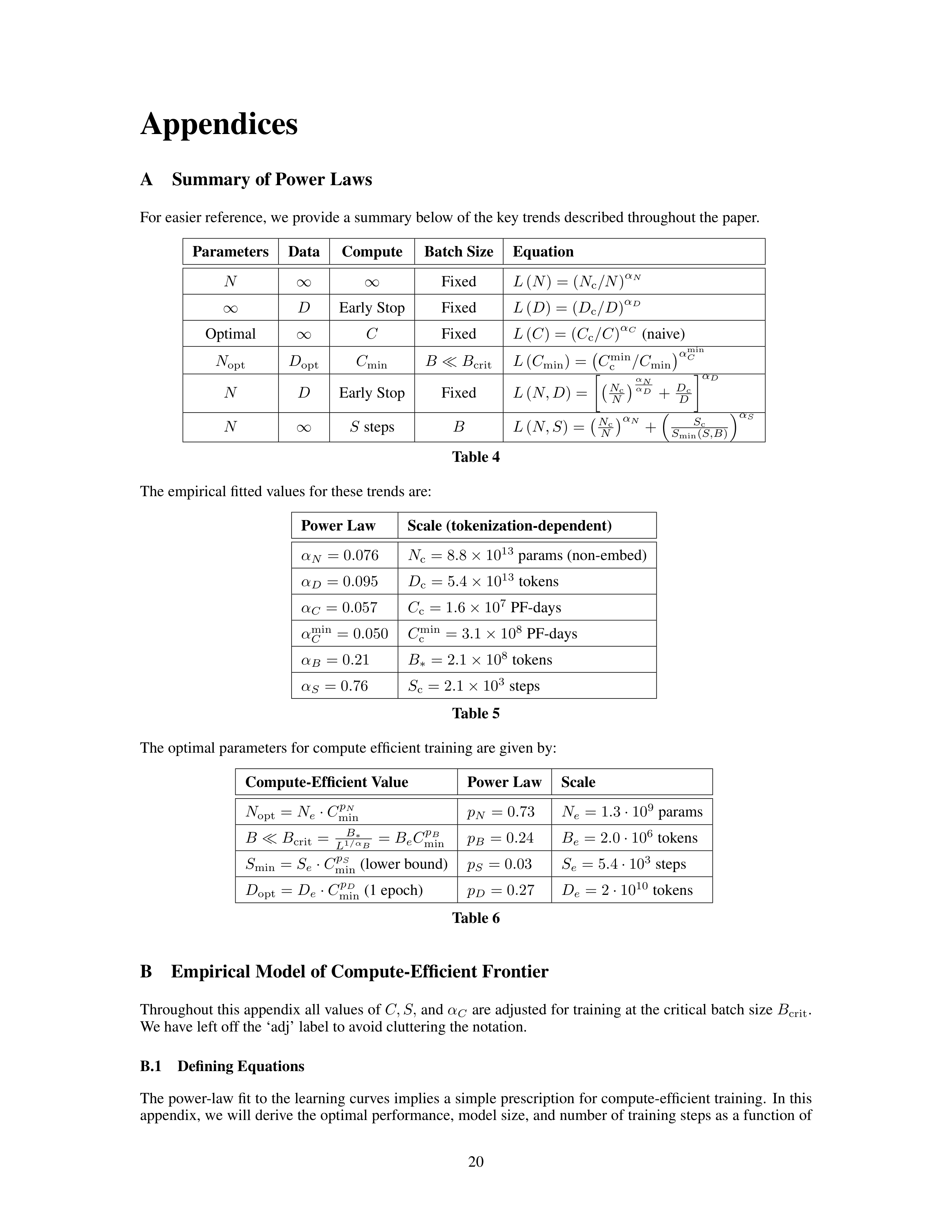
Appendices
A
Summary of Power Laws
For easier reference, we provide a summary below of the key trends described throughout the paper.
Parameters
Data
Compute
Batch Size
Equation
N
∞
∞
Fixed
L
(
N
) = (
N
c
/N
)
α
N
∞
D
Early Stop
Fixed
L
(
D
) = (
D
c
/D
)
α
D
Optimal
∞
C
Fixed
L
(
C
) = (
C
c
/C
)
α
C
(naive)
N
opt
D
opt
C
min
B
≪
B
crit
L
(
C
min
) =
C
min
c
/C
min
α
min
C
N
D
Early Stop
Fixed
L
(
N, D
) =
N
c
N
αN
αD
+
D
c
D
α
D
N
∞
S
steps
B
L
(
N, S
) =
N
c
N
α
N
+
S
c
S
min
(
S,B
)
α
S
Table 4
The empirical fitted values for these trends are:
Power Law
Scale (tokenization-dependent)
α
N
= 0
.
076
N
c
= 8
.
8
×
10
13
params (non-embed)
α
D
= 0
.
095
D
c
= 5
.
4
×
10
13
tokens
α
C
= 0
.
057
C
c
= 1
.
6
×
10
7
PF-days
α
min
C
= 0
.
050
C
min
c
= 3
.
1
×
10
8
PF-days
α
B
= 0
.
21
B
∗
= 2
.
1
×
10
8
tokens
α
S
= 0
.
76
S
c
= 2
.
1
×
10
3
steps
Table 5
The optimal parameters for compute efficient training are given by:
Compute-Efficient Value
Power Law
Scale
N
opt
=
N
e
·
C
p
N
min
p
N
= 0
.
73
N
e
= 1
.
3
·
10
9
params
B
≪
B
crit
=
B
∗
L
1
/αB
=
B
e
C
p
B
min
p
B
= 0
.
24
B
e
= 2
.
0
·
10
6
tokens
S
min
=
S
e
·
C
p
S
min
(lower bound)
p
S
= 0
.
03
S
e
= 5
.
4
·
10
3
steps
D
opt
=
D
e
·
C
p
D
min
(1 epoch)
p
D
= 0
.
27
D
e
= 2
·
10
10
tokens
Table 6
B
Empirical Model of Compute-Efficient Frontier
Throughout this appendix all values of
C, S,
and
α
C
are adjusted for training at the critical batch size
B
crit
.
We have left off the ‘adj’ label to avoid cluttering the notation.
B.1
Defining Equations
The power-law fit to the learning curves implies a simple prescription for compute-efficient training.
In this
appendix, we will derive the optimal performance, model size, and number of training steps as a function of
20
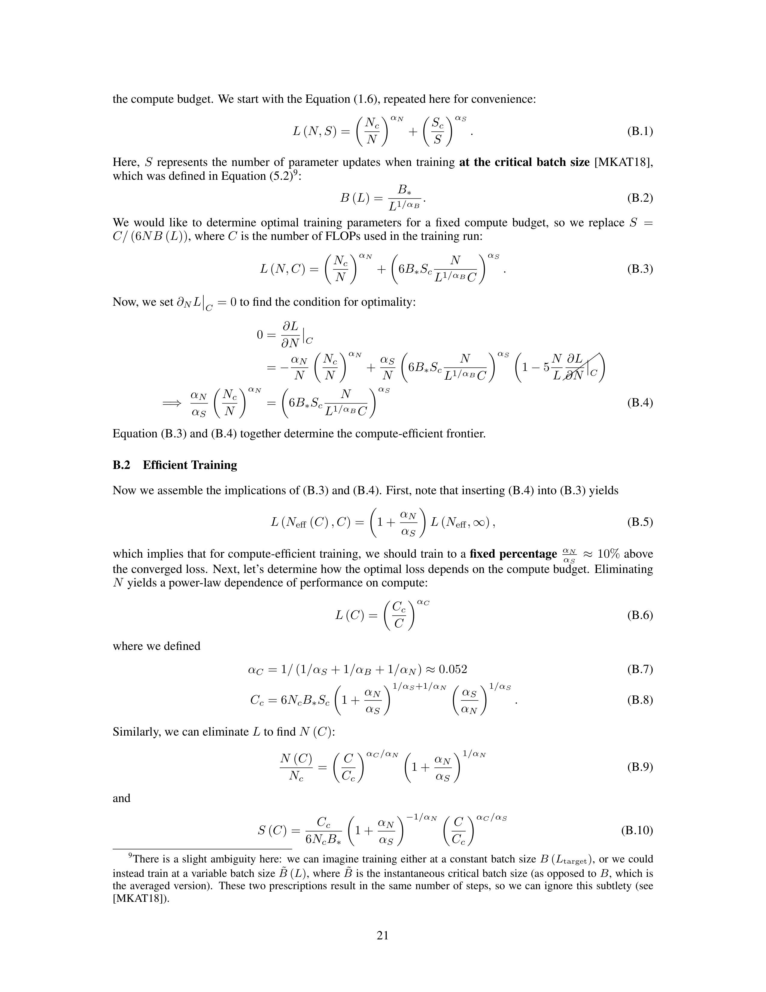
the compute budget.
We start with the Equation (1.6), repeated here for convenience:
L
(
N, S
) =
N
c
N
α
N
+
S
c
S
α
S
.
(B.1)
Here,
S
represents
the
number
of
parameter
updates
when
training
at
the
critical
batch
size
[MKAT18],
which was defined in Equation (5.2)
9
:
B
(
L
) =
B
∗
L
1
/α
B
.
(B.2)
We
would
like
to
determine
optimal
training
parameters
for
a
fixed
compute
budget,
so
we
replace
S
=
C/
(6
NB
(
L
))
, where
C
is the number of FLOPs used in the training run:
L
(
N, C
) =
N
c
N
α
N
+
6
B
∗
S
c
N
L
1
/α
B
C
α
S
.
(B.3)
Now, we set
∂
N
L
C
= 0
to find the condition for optimality:
0 =
∂L
∂N
C
=
−
α
N
N
N
c
N
α
N
+
α
S
N
6
B
∗
S
c
N
L
1
/α
B
C
α
S
1
−
5
N
L
∂L
∂N
C
=
⇒
α
N
α
S
N
c
N
α
N
=
6
B
∗
S
c
N
L
1
/α
B
C
α
S
(B.4)
Equation (B.3) and (B.4) together determine the compute-efficient frontier.
B.2
Efficient Training
Now we assemble the implications of (B.3) and (B.4).
First, note that inserting (B.4) into (B.3) yields
L
(
N
eff
(
C
)
, C
) =
1 +
α
N
α
S
L
(
N
eff
,
∞
)
,
(B.5)
which implies
that
for
compute-efficient
training,
we should train to a
fixed percentage
α
N
α
S
≈
10%
above
the converged loss.
Next, let’s determine how the optimal loss depends on the compute budget.
Eliminating
N
yields a power-law dependence of performance on compute:
L
(
C
) =
C
c
C
α
C
(B.6)
where we defined
α
C
= 1
/
(1
/α
S
+ 1
/α
B
+ 1
/α
N
)
≈
0
.
052
(B.7)
C
c
= 6
N
c
B
∗
S
c
1 +
α
N
α
S
1
/α
S
+1
/α
N
α
S
α
N
1
/α
S
.
(B.8)
Similarly, we can eliminate
L
to find
N
(
C
)
:
N
(
C
)
N
c
=
C
C
c
α
C
/α
N
1 +
α
N
α
S
1
/α
N
(B.9)
and
S
(
C
) =
C
c
6
N
c
B
∗
1 +
α
N
α
S
−
1
/α
N
C
C
c
α
C
/α
S
(B.10)
9
There
is
a
slight
ambiguity
here:
we
can
imagine
training
either
at
a
constant
batch
size
B
(
L
target
)
,
or
we
could
instead train at a variable batch size
˜
B
(
L
)
,
where
˜
B
is the instantaneous critical batch size (as opposed to
B
, which is
the
averaged
version).
These
two
prescriptions
result
in
the
same
number
of
steps,
so
we
can
ignore
this
subtlety
(see
[MKAT18]).
21
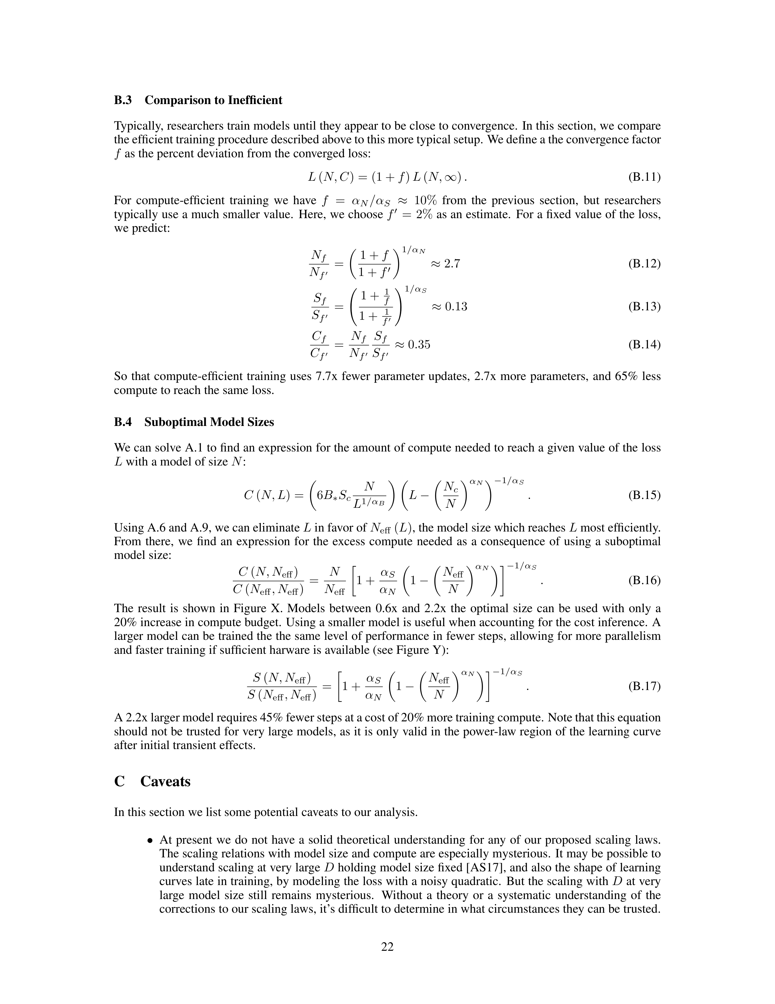
B.3
Comparison to Inefficient
Typically, researchers train models until they appear to be close to convergence.
In this section, we compare
the efficient training procedure described above to this more typical setup. We define a the convergence factor
f
as the percent deviation from the converged loss:
L
(
N, C
) = (1 +
f
)
L
(
N,
∞
)
.
(B.11)
For
compute-efficient
training
we
have
f
=
α
N
/α
S
≈
10%
from
the
previous
section,
but
researchers
typically use a much smaller value.
Here, we choose
f
′
=
2%
as an estimate.
For a fixed value of the loss,
we predict:
N
f
N
f
′
=
1 +
f
1 +
f
′
1
/α
N
≈
2
.
7
(B.12)
S
f
S
f
′
=
1 +
1
f
1 +
1
f
′
!
1
/α
S
≈
0
.
13
(B.13)
C
f
C
f
′
=
N
f
N
f
′
S
f
S
f
′
≈
0
.
35
(B.14)
So
that
compute-efficient
training
uses
7.7x
fewer
parameter
updates,
2.7x
more
parameters,
and
65%
less
compute to reach the same loss.
B.4
Suboptimal Model Sizes
We can solve A.1 to find an expression for the amount of compute needed to reach a given value of the loss
L
with a model of size
N
:
C
(
N, L
) =
6
B
∗
S
c
N
L
1
/α
B
L
−
N
c
N
α
N
−
1
/α
S
.
(B.15)
Using A.6 and A.9, we can eliminate
L
in favor of
N
eff
(
L
)
, the model size which reaches
L
most efficiently.
From
there,
we
find
an
expression
for
the
excess
compute
needed
as
a
consequence
of
using
a
suboptimal
model size:
C
(
N, N
eff
)
C
(
N
eff
, N
eff
)
=
N
N
eff
1 +
α
S
α
N
1
−
N
eff
N
α
N
−
1
/α
S
.
(B.16)
The
result
is
shown
in
Figure
X.
Models
between
0.6x
and
2.2x
the
optimal
size
can
be
used
with
only
a
20% increase in compute budget.
Using a smaller model is useful when accounting for the cost inference.
A
larger model can be trained the the same level of performance in fewer steps, allowing for more parallelism
and faster training if sufficient harware is available (see Figure Y):
S
(
N, N
eff
)
S
(
N
eff
, N
eff
)
=
1 +
α
S
α
N
1
−
N
eff
N
α
N
−
1
/α
S
.
(B.17)
A 2.2x larger model requires 45% fewer steps at a cost of 20% more training compute. Note that this equation
should not be trusted for very large models, as it is only valid in the power-law region of the learning curve
after initial transient effects.
C
Caveats
In this section we list some potential caveats to our analysis.
•
At
present
we
do
not
have
a
solid
theoretical
understanding
for
any
of
our
proposed
scaling
laws.
The scaling relations with model size and compute are especially mysterious.
It may be possible to
understand scaling at very large
D
holding model size fixed [AS17], and also the shape of learning
curves late in training, by modeling the loss with a noisy quadratic.
But the scaling with
D
at very
large
model
size
still
remains
mysterious.
Without
a
theory
or
a
systematic
understanding
of
the
corrections to our scaling laws, it’s difficult to determine in what circumstances they can be trusted.
22
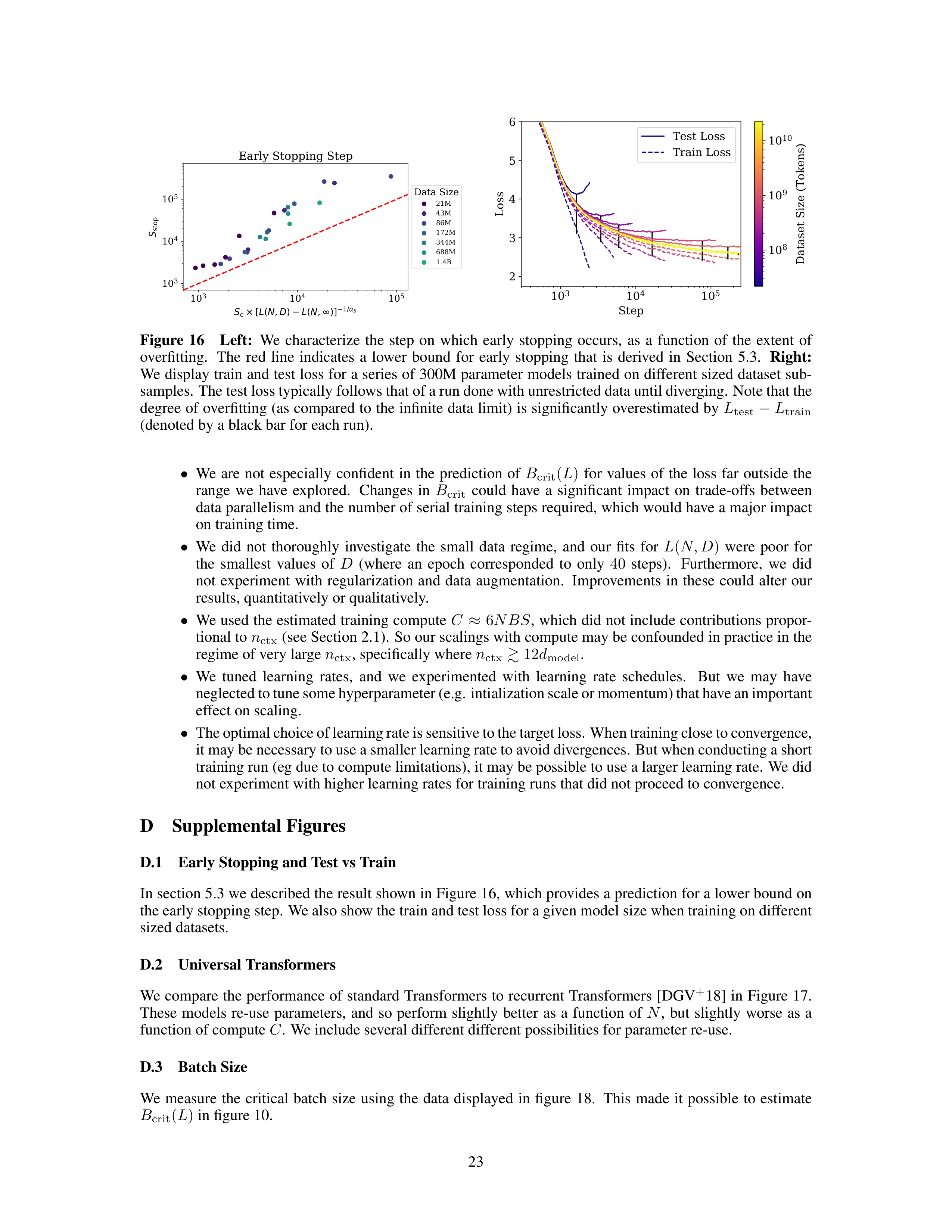

10
3
10
4
10
5
S
c
× [
L
(
N
,
D
)
L
(
N
,
)]
1/
S
10
3
10
4
10
5
S
stop
Early Stopping Step
Data Size
21M
43M
86M
172M
344M
688M
1.4B
10
3
10
4
10
5
Step
2
3
4
5
6
Loss
Test Loss
Train Loss
10
8
10
9
10
10
Dataset Size (Tokens)
Figure
16
Left:
We
characterize
the
step
on
which
early
stopping
occurs,
as
a
function
of
the
extent
of
overfitting.
The
red
line
indicates
a
lower
bound
for
early
stopping
that
is
derived
in
Section
5.3.
Right:
We display train and test loss for a series of 300M parameter models trained on different sized dataset sub-
samples.
The test loss typically follows that of a run done with unrestricted data until diverging.
Note that the
degree of overfitting (as compared to the infinite data limit) is significantly overestimated by
L
test
−
L
train
(denoted by a black bar for each run).
•
We
are
not
especially
confident
in
the
prediction
of
B
crit
(
L
)
for
values
of
the
loss
far
outside
the
range
we
have
explored.
Changes
in
B
crit
could
have
a
significant
impact
on
trade-offs
between
data parallelism and the number of serial training steps required, which would have a major impact
on training time.
•
We
did
not
thoroughly
investigate
the
small
data
regime,
and
our
fits
for
L
(
N, D
)
were
poor
for
the
smallest
values
of
D
(where
an
epoch
corresponded
to
only
40
steps).
Furthermore,
we
did
not
experiment
with
regularization
and
data
augmentation.
Improvements
in
these
could
alter
our
results, quantitatively or qualitatively.
•
We used the estimated training compute
C
≈
6
NBS
, which did not include contributions propor-
tional to
n
ctx
(see Section 2.1).
So our scalings with compute may be confounded in practice in the
regime of very large
n
ctx
, specifically where
n
ctx
≳
12
d
model
.
•
We
tuned
learning
rates,
and
we
experimented
with
learning
rate
schedules.
But
we
may
have
neglected to tune some hyperparameter (e.g. intialization scale or momentum) that have an important
effect on scaling.
•
The optimal choice of learning rate is sensitive to the target loss. When training close to convergence,
it may be necessary to use a smaller learning rate to avoid divergences.
But when conducting a short
training run (eg due to compute limitations), it may be possible to use a larger learning rate.
We did
not experiment with higher learning rates for training runs that did not proceed to convergence.
D
Supplemental Figures
D.1
Early Stopping and Test vs Train
In section 5.3 we described the result shown in Figure 16, which provides a prediction for a lower bound on
the early stopping step.
We also show the train and test loss for a given model size when training on different
sized datasets.
D.2
Universal Transformers
We compare the
performance of standard Transformers to recurrent Transformers [DGV
+
18] in Figure 17.
These
models
re-use
parameters,
and
so
perform
slightly
better
as
a
function
of
N
,
but
slightly
worse
as
a
function of compute
C
.
We include several different different possibilities for parameter re-use.
D.3
Batch Size
We
measure
the
critical
batch
size
using
the
data
displayed
in
figure
18.
This
made
it
possible
to
estimate
B
crit
(
L
)
in figure 10.
23
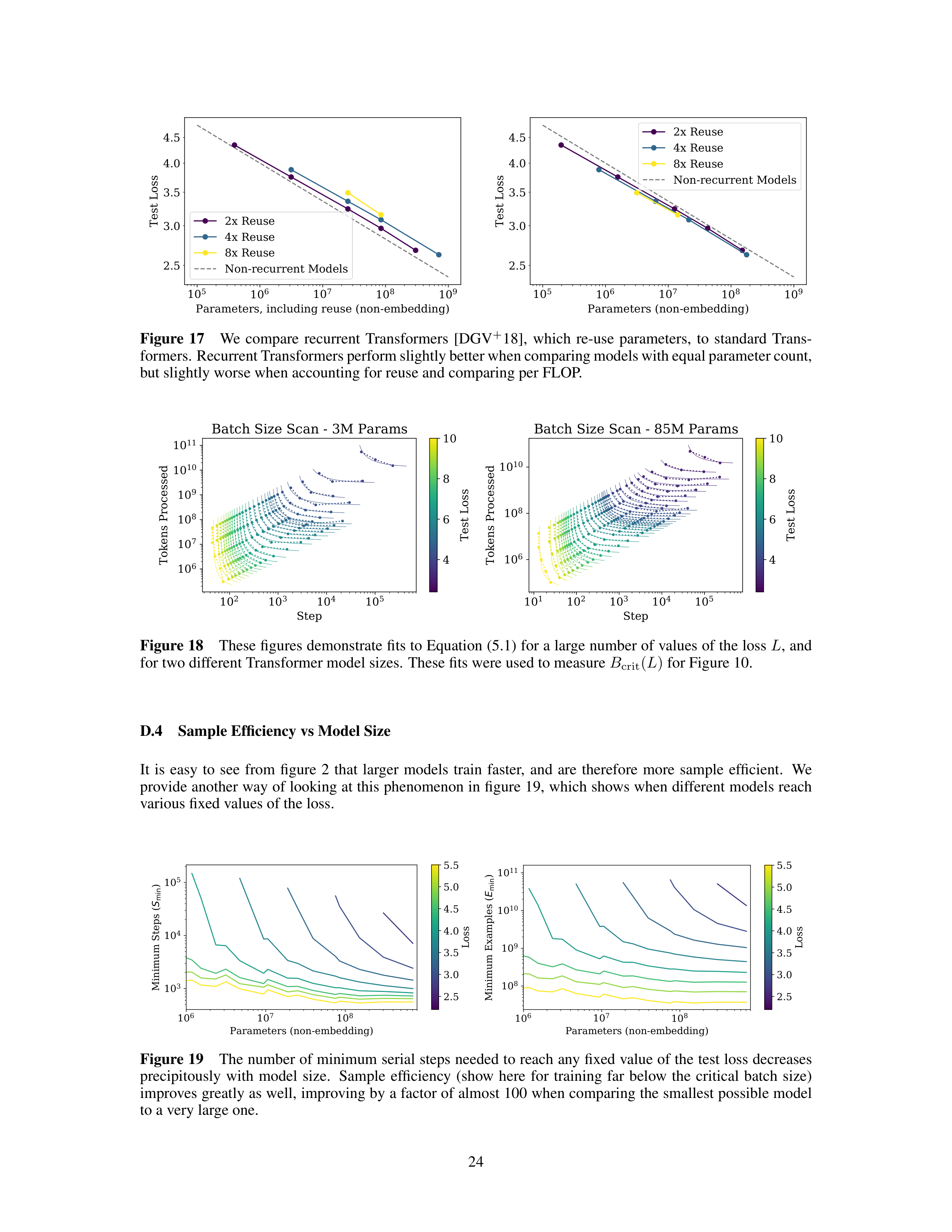




10
5
10
6
10
7
10
8
10
9
Parameters, including reuse (non-embedding)
2.5
3.0
3.5
4.0
4.5
Test Loss
2x Reuse
4x Reuse
8x Reuse
Non-recurrent Models
10
5
10
6
10
7
10
8
10
9
Parameters (non-embedding)
2.5
3.0
3.5
4.0
4.5
Test Loss
2x Reuse
4x Reuse
8x Reuse
Non-recurrent Models
Figure
17
We
compare
recurrent
Transformers
[DGV
+
18],
which
re-use
parameters,
to
standard
Trans-
formers. Recurrent Transformers perform slightly better when comparing models with equal parameter count,
but slightly worse when accounting for reuse and comparing per FLOP.
10
2
10
3
10
4
10
5
Step
10
6
10
7
10
8
10
9
10
10
10
11
Tokens Processed
Batch Size Scan - 3M Params
4
6
8
10
Test Loss
10
1
10
2
10
3
10
4
10
5
Step
10
6
10
8
10
10
Tokens Processed
Batch Size Scan - 85M Params
4
6
8
10
Test Loss
Figure 18
These figures demonstrate fits to Equation (5.1) for a large number of values of the loss
L
, and
for two different Transformer model sizes.
These fits were used to measure
B
crit
(
L
)
for Figure 10.
D.4
Sample Efficiency vs Model Size
It
is
easy
to
see
from
figure
2
that
larger
models
train
faster,
and
are
therefore
more
sample
efficient.
We
provide another way of looking at this phenomenon in figure 19, which shows when different models reach
various fixed values of the loss.
10
6
10
7
10
8
Parameters (non-embedding)
10
3
10
4
10
5
Minimum Steps (
S
min
)
2.5
3.0
3.5
4.0
4.5
5.0
5.5
Loss
10
6
10
7
10
8
Parameters (non-embedding)
10
8
10
9
10
10
10
11
Minimum Examples (
E
min
)
2.5
3.0
3.5
4.0
4.5
5.0
5.5
Loss
Figure 19
The number of minimum serial steps needed to reach any fixed value of the test loss decreases
precipitously
with
model
size.
Sample
efficiency
(show
here
for
training
far
below
the
critical
batch
size)
improves greatly as well, improving by a factor of almost 100 when comparing the smallest possible model
to a very large one.
24
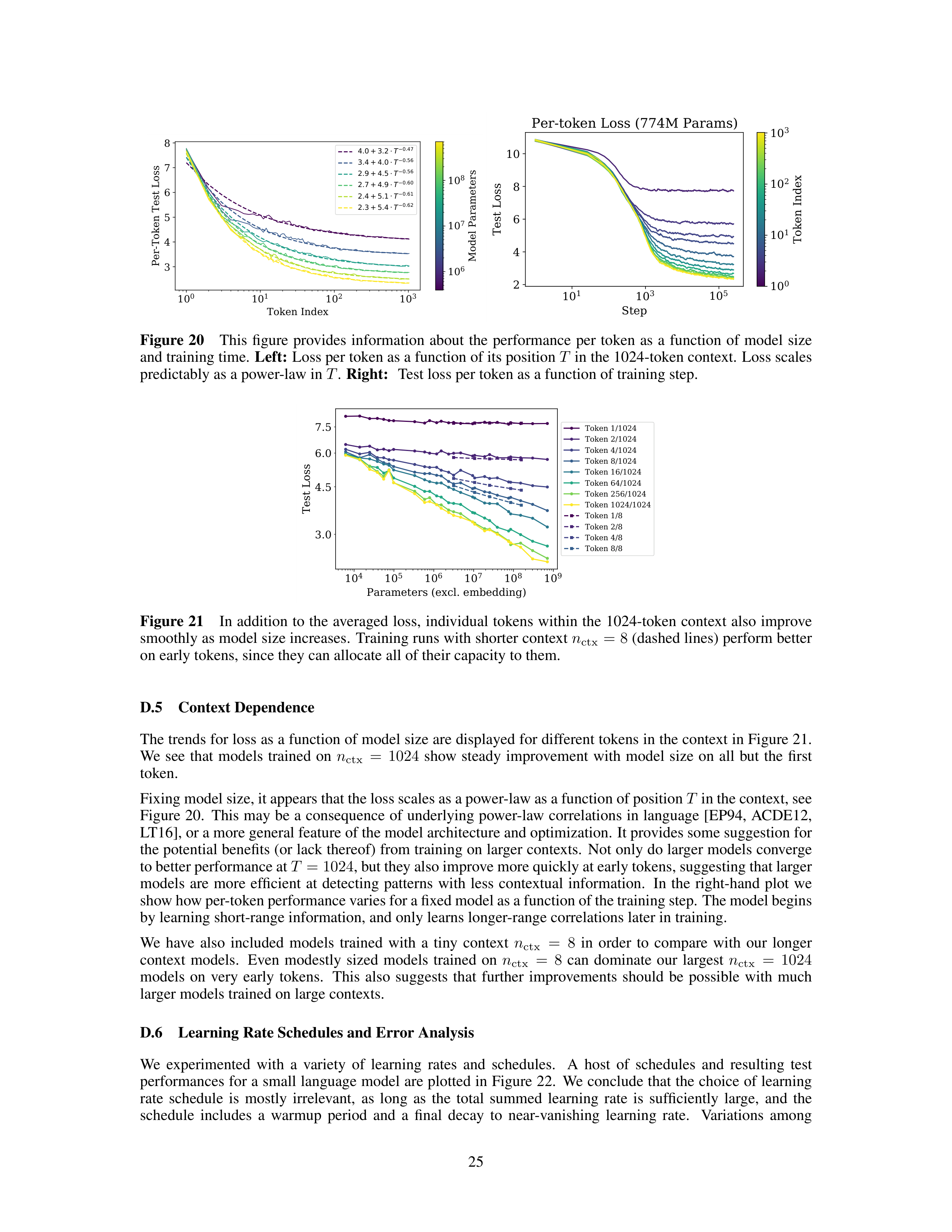


10
0
10
1
10
2
10
3
Token Index
3
4
5
6
7
8
Per-Token Test Loss
4.0 + 3.2
T
0.47
3.4 + 4.0
T
0.56
2.9 + 4.5
T
0.56
2.7 + 4.9
T
0.60
2.4 + 5.1
T
0.61
2.3 + 5.4
T
0.62
10
6
10
7
10
8
Model Parameters
10
1
10
3
10
5
Step
2
4
6
8
10
Test Loss
Per-token Loss (774M Params)
10
0
10
1
10
2
10
3
Token Index
Figure
20
This
figure
provides
information
about
the
performance
per
token
as
a
function
of
model
size
and training time.
Left:
Loss per token as a function of its position
T
in the 1024-token context.
Loss scales
predictably as a power-law in
T
.
Right:
Test loss per token as a function of training step.
10
4
10
5
10
6
10
7
10
8
10
9
Parameters (excl. embedding)
3.0
4.5
6.0
7.5
Test Loss
Token 1/1024
Token 2/1024
Token 4/1024
Token 8/1024
Token 16/1024
Token 64/1024
Token 256/1024
Token 1024/1024
Token 1/8
Token 2/8
Token 4/8
Token 8/8
Figure
21
In
addition
to
the
averaged
loss,
individual
tokens
within
the
1024-token
context
also
improve
smoothly as model size increases.
Training runs with shorter context
n
ctx
=
8
(dashed lines) perform better
on early tokens, since they can allocate all of their capacity to them.
D.5
Context Dependence
The trends for loss as a function of model size are displayed for different tokens in the context in Figure 21.
We
see
that
models
trained
on
n
ctx
=
1024
show
steady
improvement
with
model
size
on
all
but
the
first
token.
Fixing model size, it appears that the loss scales as a power-law as a function of position
T
in the context, see
Figure 20.
This may be a consequence of underlying power-law correlations in language [EP94, ACDE12,
LT16], or a more general feature of the model architecture and optimization.
It provides some suggestion for
the potential benefits (or lack thereof) from training on larger contexts.
Not only do larger models converge
to better performance at
T
= 1024
, but they also improve more quickly at early tokens, suggesting that larger
models
are
more
efficient
at
detecting
patterns
with
less
contextual
information.
In
the
right-hand
plot
we
show how per-token performance varies for a fixed model as a function of the training step. The model begins
by learning short-range information, and only learns longer-range correlations later in training.
We
have
also
included
models
trained
with
a
tiny
context
n
ctx
=
8
in
order
to
compare
with
our
longer
context
models.
Even
modestly
sized
models
trained
on
n
ctx
=
8
can
dominate
our
largest
n
ctx
=
1024
models
on
very
early
tokens.
This
also
suggests
that
further
improvements
should
be
possible
with
much
larger models trained on large contexts.
D.6
Learning Rate Schedules and Error Analysis
We
experimented
with
a
variety
of
learning
rates
and
schedules.
A
host
of
schedules
and
resulting
test
performances for a small language model are plotted in Figure 22.
We conclude that the choice of learning
rate
schedule
is
mostly
irrelevant,
as
long
as
the
total
summed
learning
rate
is
sufficiently
large,
and
the
schedule
includes
a
warmup
period
and
a
final
decay
to
near-vanishing
learning
rate.
Variations
among
25
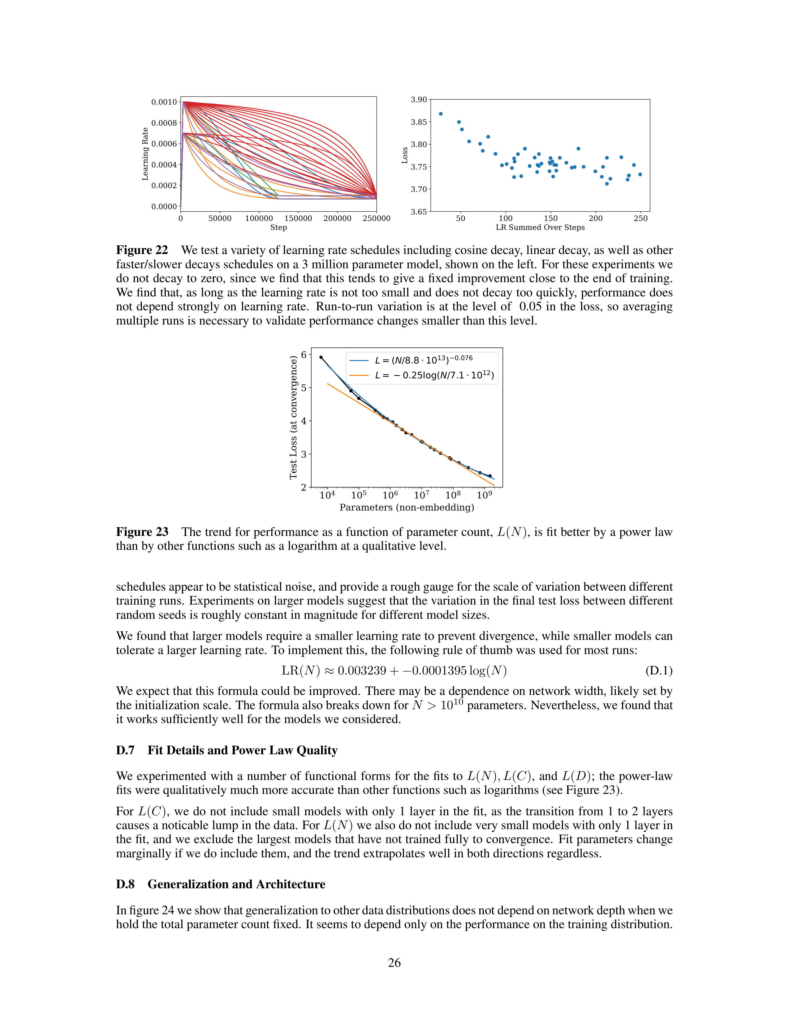
0
50000
100000
150000
200000
250000
Step
0.0000
0.0002
0.0004
0.0006
0.0008
0.0010
Learning Rate
50
100
150
200
250
LR Summed Over Steps
3.65
3.70
3.75
3.80
3.85
3.90
Loss
Figure 22
We test a variety of learning rate schedules including cosine decay, linear decay, as well as other
faster/slower decays schedules on a 3 million parameter model, shown on the left.
For these experiments we
do not decay to zero,
since we find that this tends to give a fixed improvement close to the end of training.
We find that, as long as the learning rate is not too small and does not decay too quickly, performance does
not
depend
strongly
on
learning
rate.
Run-to-run
variation
is
at
the
level
of
0.05
in
the
loss,
so
averaging
multiple runs is necessary to validate performance changes smaller than this level.
10
4
10
5
10
6
10
7
10
8
10
9
Parameters (non-embedding)
2
3
4
5
6
Test Loss (at convergence)
L
= (
N
/8.8
10
13
)
0.076
L
=
0.25log(
N
/7.1
10
12
)
Figure 23
The trend for performance as a function of parameter count,
L
(
N
)
, is fit better by a power law
than by other functions such as a logarithm at a qualitative level.
schedules appear to be statistical noise, and provide a rough gauge for the scale of variation between different
training runs.
Experiments on larger models suggest that the variation in the final test loss between different
random seeds is roughly constant in magnitude for different model sizes.
We found that larger models require a smaller learning rate to prevent divergence, while smaller models can
tolerate a larger learning rate.
To implement this, the following rule of thumb was used for most runs:
LR(
N
)
≈
0
.
003239 +
−
0
.
0001395 log(
N
)
(D.1)
We expect that this formula could be improved.
There may be a dependence on network width, likely set by
the initialization scale.
The formula also breaks down for
N
>
10
10
parameters.
Nevertheless, we found that
it works sufficiently well for the models we considered.
D.7
Fit Details and Power Law Quality
We
experimented
with
a
number
of
functional
forms
for
the
fits
to
L
(
N
)
, L
(
C
)
,
and
L
(
D
)
;
the
power-law
fits were qualitatively much more accurate than other functions such as logarithms (see Figure 23).
For
L
(
C
)
,
we
do
not
include
small
models
with
only
1
layer
in
the
fit,
as
the
transition
from
1
to
2
layers
causes a noticable lump in the data.
For
L
(
N
)
we also do not include very small models with only 1 layer in
the fit, and we exclude the largest models that have not trained fully to convergence.
Fit parameters change
marginally if we do include them, and the trend extrapolates well in both directions regardless.
D.8
Generalization and Architecture
In figure 24 we show that generalization to other data distributions does not depend on network depth when we
hold the total parameter count fixed.
It seems to depend only on the performance on the training distribution.
26
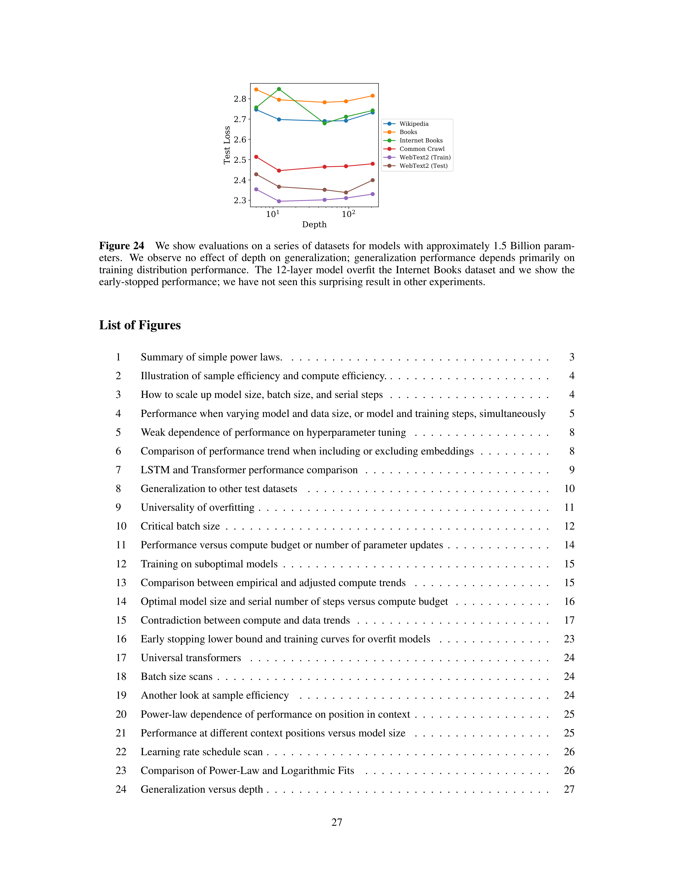
10
1
10
2
Depth
2.3
2.4
2.5
2.6
2.7
2.8
Test Loss
Wikipedia
Books
Internet Books
Common Crawl
WebText2 (Train)
WebText2 (Test)
Figure 24
We show evaluations on a series of datasets for models with approximately 1.5 Billion param-
eters.
We
observe
no
effect
of
depth
on
generalization;
generalization
performance
depends
primarily
on
training
distribution
performance.
The
12-layer
model
overfit
the
Internet
Books
dataset
and
we
show
the
early-stopped performance; we have not seen this surprising result in other experiments.
List of Figures
1
Summary of simple power laws.
.
.
.
.
.
.
.
.
.
.
.
.
.
.
.
.
.
.
.
.
.
.
.
.
.
.
.
.
.
.
.
.
3
2
Illustration of sample efficiency and compute efficiency. .
.
.
.
.
.
.
.
.
.
.
.
.
.
.
.
.
.
.
.
4
3
How to scale up model size, batch size, and serial steps
.
.
.
.
.
.
.
.
.
.
.
.
.
.
.
.
.
.
.
.
4
4
Performance when varying model and data size, or model and training steps, simultaneously
5
5
Weak dependence of performance on hyperparameter tuning
.
.
.
.
.
.
.
.
.
.
.
.
.
.
.
.
.
8
6
Comparison of performance trend when including or excluding embeddings
.
.
.
.
.
.
.
.
.
8
7
LSTM and Transformer performance comparison
.
.
.
.
.
.
.
.
.
.
.
.
.
.
.
.
.
.
.
.
.
.
.
9
8
Generalization to other test datasets
.
.
.
.
.
.
.
.
.
.
.
.
.
.
.
.
.
.
.
.
.
.
.
.
.
.
.
.
.
.
10
9
Universality of overfitting
.
.
.
.
.
.
.
.
.
.
.
.
.
.
.
.
.
.
.
.
.
.
.
.
.
.
.
.
.
.
.
.
.
.
.
.
11
10
Critical batch size
.
.
.
.
.
.
.
.
.
.
.
.
.
.
.
.
.
.
.
.
.
.
.
.
.
.
.
.
.
.
.
.
.
.
.
.
.
.
.
.
12
11
Performance versus compute budget or number of parameter updates
.
.
.
.
.
.
.
.
.
.
.
.
.
14
12
Training on suboptimal models
.
.
.
.
.
.
.
.
.
.
.
.
.
.
.
.
.
.
.
.
.
.
.
.
.
.
.
.
.
.
.
.
.
15
13
Comparison between empirical and adjusted compute trends
.
.
.
.
.
.
.
.
.
.
.
.
.
.
.
.
.
15
14
Optimal model size and serial number of steps versus compute budget
.
.
.
.
.
.
.
.
.
.
.
.
16
15
Contradiction between compute and data trends
.
.
.
.
.
.
.
.
.
.
.
.
.
.
.
.
.
.
.
.
.
.
.
.
17
16
Early stopping lower bound and training curves for overfit models
.
.
.
.
.
.
.
.
.
.
.
.
.
.
23
17
Universal transformers
.
.
.
.
.
.
.
.
.
.
.
.
.
.
.
.
.
.
.
.
.
.
.
.
.
.
.
.
.
.
.
.
.
.
.
.
.
24
18
Batch size scans
.
.
.
.
.
.
.
.
.
.
.
.
.
.
.
.
.
.
.
.
.
.
.
.
.
.
.
.
.
.
.
.
.
.
.
.
.
.
.
.
.
24
19
Another look at sample efficiency
.
.
.
.
.
.
.
.
.
.
.
.
.
.
.
.
.
.
.
.
.
.
.
.
.
.
.
.
.
.
.
24
20
Power-law dependence of performance on position in context
.
.
.
.
.
.
.
.
.
.
.
.
.
.
.
.
.
25
21
Performance at different context positions versus model size
.
.
.
.
.
.
.
.
.
.
.
.
.
.
.
.
.
25
22
Learning rate schedule scan
.
.
.
.
.
.
.
.
.
.
.
.
.
.
.
.
.
.
.
.
.
.
.
.
.
.
.
.
.
.
.
.
.
.
.
26
23
Comparison of Power-Law and Logarithmic Fits
.
.
.
.
.
.
.
.
.
.
.
.
.
.
.
.
.
.
.
.
.
.
.
26
24
Generalization versus depth
.
.
.
.
.
.
.
.
.
.
.
.
.
.
.
.
.
.
.
.
.
.
.
.
.
.
.
.
.
.
.
.
.
.
.
27
27

List of Tables
1
Parameter and compute counts for Transformer
.
.
.
.
.
.
.
.
.
.
.
.
.
.
.
.
.
.
.
.
.
.
.
.
7
2
Fits to
L
(
N, D
)
.
.
.
.
.
.
.
.
.
.
.
.
.
.
.
.
.
.
.
.
.
.
.
.
.
.
.
.
.
.
.
.
.
.
.
.
.
.
.
.
.
11
3
Fits to
L
(
N, S
)
.
.
.
.
.
.
.
.
.
.
.
.
.
.
.
.
.
.
.
.
.
.
.
.
.
.
.
.
.
.
.
.
.
.
.
.
.
.
.
.
.
14
4
Key trend equations
.
.
.
.
.
.
.
.
.
.
.
.
.
.
.
.
.
.
.
.
.
.
.
.
.
.
.
.
.
.
.
.
.
.
.
.
.
.
.
20
5
Key parameters to trend fits
.
.
.
.
.
.
.
.
.
.
.
.
.
.
.
.
.
.
.
.
.
.
.
.
.
.
.
.
.
.
.
.
.
.
.
20
6
Trends for compute-efficient training
.
.
.
.
.
.
.
.
.
.
.
.
.
.
.
.
.
.
.
.
.
.
.
.
.
.
.
.
.
.
20
References
[ACDE12]
Eduardo
G
Altmann,
Giampaolo
Cristadoro,
and
Mirko
Degli
Esposti.
On
the
origin
of
long-
range correlations in texts.
Proceedings of the National Academy of Sciences
, 109(29):11582–
11587, 2012.
25
[AS17]
Madhu S. Advani and Andrew M. Saxe.
High-dimensional dynamics of generalization error in
neural networks.
arXiv
, 2017, 1710.03667.
11, 18, 22
[BB01]
Michele
Banko
and
Eric
Brill.
Scaling
to
very
very
large
corpora
for
natural
language
disam-
biguation.
In
Proceedings of the 39th annual meeting on association for computational linguis-
tics
, pages 26–33. Association for Computational Linguistics, 2001.
18
[BHMM18]
Mikhail
Belkin,
Daniel
Hsu,
Siyuan
Ma,
and
Soumik
Mandal.
Reconciling
modern
machine
learning and the bias-variance trade-off.
arXiv
, 2018, 1812.11118.
18
[Bia12]
GÊrard
Biau.
Analysis
of
a
random
forests
model.
Journal
of
Machine
Learning
Research
,
13(Apr):1063–1095, 2012.
18
[CGRS19]
Rewon
Child,
Scott
Gray,
Alec
Radford,
and
Ilya
Sutskever.
Generating
long
sequences
with
sparse
transformers.
CoRR
,
abs/1904.10509,
2019,
1904.10509.
URL
http://arxiv.org/
abs/1904.10509
.
19
[DCLT18]
Jacob Devlin, Ming-Wei Chang, Kenton Lee, and Kristina Toutanova. Bert: Pre-training of deep
bidirectional transformers for language understanding, 2018, arXiv:1810.04805.
2
[DGV
+
18]
Mostafa
Dehghani,
Stephan
Gouws,
Oriol
Vinyals,
Jakob
Uszkoreit,
and
Lukasz
Kaiser.
Uni-
versal
transformers.
CoRR
,
abs/1807.03819,
2018,
1807.03819.
URL
http://arxiv.org/
abs/1807.03819
.
6, 9, 23, 24
[EP94]
Werner Ebeling and Thorsten Pöschel.
Entropy and long-range correlations in literary english.
EPL (Europhysics Letters)
, 26(4):241, 1994.
25
[Fou]
The Common Crawl Foundation.
Common crawl.
URL
http://commoncrawl.org
.
7
[GARD18]
Guy Gur-Ari, Daniel A. Roberts, and Ethan Dyer.
Gradient descent happens in a tiny subspace.
2018, arXiv:1812.04754.
18
[GJS
+
19]
Mario Geiger, Arthur Jacot, Stefano Spigler, Franck Gabriel, Levent Sagun, Stéphane d’Ascoli,
Giulio Biroli, Clément Hongler, and Matthieu Wyart.
Scaling description of generalization with
number of parameters in deep learning.
arXiv
, 2019, 1901.01608.
18
[GKX19]
Behrooz
Ghorbani,
Shankar
Krishnan,
and
Ying
Xiao.
An
investigation
into
neural
net
op-
timization
via
hessian
eigenvalue
density.
CoRR
,
abs/1901.10159,
2019,
1901.10159.
URL
http://arxiv.org/abs/1901.10159
.
18
[Goo01]
Joshua Goodman.
A bit of progress in language modeling.
CoRR
, cs.CL/0108005, 2001.
URL
http://arxiv.org/abs/cs.CL/0108005
.
18
[GRK17]
Scott Gray, Alec Radford, and Diederik P Kingma.
Gpu kernels for block-sparse weights.
ope-
nai.com
, 2017.
19
[HAD19]
Joel Hestness, Newsha Ardalani, and Gregory Diamos.
Beyond human-level accuracy:
Compu-
tational challenges in deep learning.
In
Proceedings of the 24th Symposium on Principles and
Practice of Parallel Programming
, PPoPP ’19, pages 1–14, New York, NY, USA, 2019. ACM.
doi:10.1145/3293883.3295710.
18
28
[HCC
+
18]
Yanping Huang, Yonglong Cheng, Dehao Chen, HyoukJoong Lee, Jiquan Ngiam, Quoc V. Le,
and Zhifeng Chen.
Gpipe: Efficient training of giant neural networks using pipeline parallelism.
CoRR
, abs/1811.06965, 2018, 1811.06965.
URL
http://arxiv.org/abs/1811.06965
.
19
[HNA
+
17]
Joel
Hestness,
Sharan
Narang,
Newsha
Ardalani,
Gregory
Diamos,
Heewoo
Jun,
Hassan
Kia-
ninejad, Md. Mostofa Ali Patwary, Yang Yang, and Yanqi Zhou.
Deep learning scaling is pre-
dictable, empirically, 2017, 1712.00409.
18
[JGH18]
Arthur
Jacot,
Franck
Gabriel,
and
Clément
Hongler.
Neural
tangent
kernel:
Convergence
and
generalization in neural networks.
In
Advances in neural information processing systems
, pages
8571–8580, 2018.
18
[KB14]
Diederik
P.
Kingma
and
Jimmy
Ba.
Adam:
A
method
for
stochastic
optimization,
2014,
1412.6980.
7
[Kom19]
Aran Komatsuzaki.
One epoch is all you need, 2019, arXiv:1906.06669.
18
[KSH12]
Alex
Krizhevsky,
Ilya
Sutskever,
and
Geoffrey
E.
Hinton.
Imagenet
classification
with
deep
convolutional neural networks.
In
Proceedings of the 25th International Conference on Neural
Information
Processing
Systems
-
Volume
1
,
NIPS’12,
pages
1097–1105,
USA,
2012.
Curran
Associates Inc.
URL
http://dl.acm.org/citation.cfm?id=2999134.2999257
.
19
[LCG
+
19]
Zhenzhong Lan, Mingda Chen, Sebastian Goodman, Kevin Gimpel, Piyush Sharma, and Radu
Soricut.
Albert:
A
lite
bert
for
self-supervised
learning
of
language
representations,
2019,
1909.11942.
9
[LOG
+
19]
Yinhan Liu, Myle Ott, Naman Goyal, Jingfei Du, Mandar Joshi, Danqi Chen, Omer Levy, Mike
Lewis, Luke Zettlemoyer, and Veselin Stoyanov.
Roberta: A robustly optimized BERT pretrain-
ing
approach.
CoRR
,
abs/1907.11692,
2019,
1907.11692.
URL
http://arxiv.org/abs/
1907.11692
.
2
[LSP
+
18]
Peter J. Liu, Mohammad Saleh, Etienne Pot, Ben Goodrich, Ryan Sepassi, Lukasz Kaiser, and
Noam Shazeer.
Generating wikipedia by summarizing long sequences.
arXiv:1801.10198 [cs]
,
2018, 1801.10198.
URL
http://arxiv.org/abs/1801.10198
.
2, 6
[LT16]
Henry W Lin and Max Tegmark.
Criticality in formal languages and statistical physics.
arXiv
preprint arXiv:1606.06737
, 2016.
25
[LXS
+
19]
Jaehoon Lee, Lechao Xiao, Samuel S. Schoenholz, Yasaman Bahri, Roman Novak, Jascha Sohl-
Dickstein, and Jeffrey Pennington.
Wide neural networks of any depth evolve as linear models
under gradient descent, 2019, arXiv:1902.06720.
18
[MKAT18]
Sam McCandlish, Jared Kaplan, Dario Amodei, and OpenAI Dota Team.
An empirical model
of large-batch training, 2018, arXiv:1812.06162.
3, 5, 6, 12, 13, 21
[Pap18]
Vardan
Papyan.
The
full
spectrum
of
deep
net
hessians
at
scale:
Dynamics
with
sample
size.
CoRR
, abs/1811.07062, 2018, 1811.07062.
URL
http://arxiv.org/abs/1811.07062
.
18
[RNSS18]
Alec
Radford,
Karthik
Narasimhan,
Tim
Salimans,
and
Ilya
Sutskever.
Improving
language
understanding
by
generative
pre-training.
URL
https://s3-us-west-2.
amazonaws.
com/openai-
assets/research-covers/languageunsupervised/language understanding paper. pdf
, 2018.
2, 6
[RRBS19a]
Jonathan
S.
Rosenfeld,
Amir
Rosenfeld,
Yonatan
Belinkov,
and
Nir
Shavit.
A
constructive
prediction of the generalization error across scales, 2019, 1909.12673.
18
[RRBS19b]
Jonathan
S.
Rosenfeld,
Amir
Rosenfeld,
Yonatan
Belinkov,
and
Nir
Shavit.
A
constructive
prediction of the generalization error across scales, 2019, arXiv:1909.12673.
18
[RSR
+
19]
Colin
Raffel,
Noam
Shazeer,
Adam
Roberts,
Katherine
Lee,
Sharan
Narang,
Michael
Matena,
Yanqi
Zhou,
Wei
Li,
and
Peter
J.
Liu.
Exploring
the
limits
of
transfer
learning
with
a
unified
text-to-text transformer, 2019, arXiv:1910.10683.
2
[RWC
+
19]
Alec Radford, Jeff Wu, Rewon Child, David Luan, Dario Amodei, and Ilya Sutskever. Language
models are unsupervised multitask learners.
openai.com
, 2019.
2, 5, 6, 7, 8
[SCP
+
18]
Noam Shazeer,
Youlong Cheng,
Niki Parmar,
Dustin Tran,
Ashish Vaswani,
Penporn Koanan-
takool,
Peter
Hawkins,
HyoukJoong
Lee,
Mingsheng
Hong,
Cliff
Young,
Ryan
Sepassi,
and
Blake Hechtman.
Mesh-tensorflow:
Deep learning for supercomputers, 2018, 1811.02084.
19
[SHB15]
Rico Sennrich, Barry Haddow, and Alexandra Birch.
Neural machine translation of rare words
with subword units.
CoRR
, 2015, 1508.07909.
6
29
[SLA
+
18]
Christopher
J.
Shallue,
Jaehoon
Lee,
Joe
Antognini,
Jascha
Sohl-Dickstein,
Roy
Frostig,
and
George
E.
Dahl.
Measuring
the
effects
of
data
parallelism
on
neural
network
training,
2018,
arXiv:1811.03600.
12
[SS18]
Noam Shazeer and Mitchell Stern.
Adafactor:
Adaptive learning rates with sublinear memory
cost.
CoRR
, abs/1804.04235, 2018, 1804.04235. URL
http://arxiv.org/abs/1804.04235
.
7
[THK18]
Stefan Thurner, Rudolf Hanel, and Peter Klimek.
Introduction to the theory of complex systems
.
Oxford University Press, 2018.
18
[TL19]
Mingxing Tan and Quoc V. Le.
Efficientnet:
Rethinking model scaling for convolutional neural
networks.
CoRR
, abs/1905.11946, 2019, 1905.11946.
URL
http://arxiv.org/abs/1905.
11946
.
18
[VSP
+
17]
Ashish
Vaswani,
Noam
Shazeer,
Niki Parmar,
Jakob Uszkoreit,
Llion Jones,
Aidan N Gomez,
Ł
ukasz
Kaiser,
and
Illia
Polosukhin.
Attention
is
all
you
need.
In
I.
Guyon,
U.
V.
Luxburg,
S. Bengio, H. Wallach, R. Fergus, S. Vishwanathan, and R. Garnett, editors,
Advances in Neural
Information
Processing
Systems
30
,
pages
5998–6008.
Curran
Associates,
Inc.,
2017.
URL
http://papers.nips.cc/paper/7181-attention-is-all-you-need.pdf
.
2, 6
[VWB16]
Andreas
Veit,
Michael
Wilber,
and
Serge Belongie.
Residual networks
behave like ensembles
of relatively shallow networks, 2016, arXiv:1605.06431.
8, 18
[Was06]
Larry Wasserman.
All of nonparametric statistics
.
Springer Science & Business Media, 2006.
18
[WPN
+
19]
Alex Wang, Yada Pruksachatkun, Nikita Nangia, Amanpreet Singh, Julian Michael, Felix Hill,
Omer
Levy,
and
Samuel
R.
Bowman.
Superglue:
A
stickier
benchmark
for
general-purpose
language understanding systems, 2019, 1905.00537.
2
[WRH17]
Yu-Xiong
Wang,
Deva
Ramanan,
and
Martial
Hebert.
Growing
a
brain:
Fine-tuning
by
in-
creasing model capacity.
2017 IEEE Conference on Computer Vision and Pattern Recognition
(CVPR)
, Jul 2017.
doi:10.1109/cvpr.2017.323.
19
[WYL19]
Wei
Wen,
Feng
Yan,
and
Hai
Li.
Autogrow:
Automatic
layer
growing
in
deep
convolutional
networks, 2019, 1906.02909.
19
[YDY
+
19]
Zhilin
Yang,
Zihang
Dai,
Yiming
Yang,
Jaime
Carbonell,
Ruslan
Salakhutdinov,
and
Quoc
V.
Le.
Xlnet:
Generalized
autoregressive
pretraining
for
language
understanding,
2019,
arXiv:1906.08237.
2
[ZK16]
Sergey
Zagoruyko
and
Nikos
Komodakis.
Wide
residual
networks.
Procedings
of
the
British
Machine Vision Conference 2016
, 2016.
doi:10.5244/c.30.87.
18
[ZKZ
+
15]
Yukun
Zhu,
Ryan
Kiros,
Rich
Zemel,
Ruslan
Salakhutdinov,
Raquel
Urtasun,
Antonio
Tor-
ralba, and Sanja Fidler.
Aligning books and movies:
Towards story-like visual explanations by
watching movies and reading books.
2015 IEEE International Conference on Computer Vision
(ICCV)
, Dec 2015.
doi:10.1109/iccv.2015.11.
7
[ZLN
+
19]
Guodong
Zhang,
Lala
Li,
Zachary
Nado,
James
Martens,
Sushant
Sachdeva,
George
E.
Dahl,
Christopher J. Shallue, and Roger B. Grosse.
Which algorithmic choices matter at which batch
sizes?
insights from a noisy quadratic model.
CoRR
, abs/1907.04164, 2019, 1907.04164.
URL
http://arxiv.org/abs/1907.04164
.
12, 18
30