ImageNet Classification with Deep Convolutional
Neural Networks
Alex Krizhevsky
University of Toronto
kriz@cs.utoronto.ca
Ilya Sutskever
University of Toronto
ilya@cs.utoronto.ca
Geoffrey E. Hinton
University of Toronto
hinton@cs.utoronto.ca
Abstract
We trained a large,
deep convolutional neural network to classify the 1.2 million
high-resolution
images
in
the
ImageNet
LSVRC-2010
contest
into
the
1000
dif-
ferent classes.
On the test data, we achieved top-1 and top-5 error rates of 37.5%
and
17.0%
which
is
considerably
better
than
the
previous
state-of-the-art.
The
neural
network,
which
has
60
million
parameters
and
650,000
neurons,
consists
of five convolutional layers,
some of which are followed by max-pooling layers,
and
three
fully-connected
layers
with
a
final
1000-way
softmax.
To
make
train-
ing
faster,
we
used
non-saturating
neurons
and
a
very
efficient
GPU
implemen-
tation
of
the
convolution
operation.
To
reduce
overfitting
in
the
fully-connected
layers we employed a recently-developed regularization method called “dropout”
that
proved
to
be
very
effective.
We
also
entered
a
variant
of
this
model
in
the
ILSVRC-2012 competition and achieved a winning top-5 test error rate of 15.3%,
compared to 26.2% achieved by the second-best entry.
1
Introduction
Current approaches to object recognition make essential use of machine learning methods.
To im-
prove
their
performance,
we
can
collect
larger
datasets,
learn
more
powerful
models,
and
use
bet-
ter techniques
for preventing
overfitting.
Until recently,
datasets of labeled images were relatively
small — on the order of tens of thousands of images (e.g., NORB [16], Caltech-101/256 [8, 9], and
CIFAR-10/100
[12]).
Simple
recognition
tasks
can
be
solved
quite
well
with
datasets
of
this
size,
especially
if
they
are
augmented
with
label-preserving
transformations.
For
example,
the
current-
best
error
rate
on
the
MNIST
digit-recognition
task
(<0.3%)
approaches
human
performance
[4].
But
objects
in
realistic
settings
exhibit
considerable
variability,
so
to
learn
to
recognize
them
it
is
necessary
to
use
much
larger
training
sets.
And
indeed,
the
shortcomings
of
small
image
datasets
have been widely recognized (e.g., Pinto et al. [21]), but it has only recently become possible to col-
lect labeled datasets with millions of images.
The new larger datasets include LabelMe [23], which
consists of hundreds of thousands of fully-segmented images, and ImageNet [6], which consists of
over 15 million labeled high-resolution images in over 22,000 categories.
To learn about thousands of objects from millions of images, we need a model with a large learning
capacity.
However,
the
immense
complexity
of
the
object
recognition
task
means
that
this
prob-
lem cannot be specified even by a dataset as large as ImageNet, so our model should also have lots
of
prior
knowledge
to
compensate
for
all
the
data
we
don’t
have.
Convolutional
neural
networks
(CNNs) constitute one such class of models [16, 11, 13, 18, 15, 22, 26].
Their capacity can be con-
trolled by varying their depth and breadth, and they also make strong and mostly correct assumptions
about
the
nature
of
images
(namely,
stationarity
of
statistics
and
locality
of
pixel
dependencies).
Thus,
compared
to
standard
feedforward
neural
networks
with
similarly-sized
layers,
CNNs
have
much fewer connections and parameters and so they are easier to train, while their theoretically-best
performance is likely to be only slightly worse.
1
Despite the attractive qualities of CNNs, and despite the relative efficiency of their local architecture,
they have still been prohibitively expensive to apply in large scale to high-resolution images.
Luck-
ily, current GPUs, paired with a highly-optimized implementation of 2D convolution, are powerful
enough to facilitate the training of interestingly-large CNNs, and recent datasets such as ImageNet
contain enough labeled examples to train such models without severe overfitting.
The specific contributions of this paper are as follows:
we trained one of the largest convolutional
neural
networks
to
date
on
the
subsets
of ImageNet
used in
the
ILSVRC-2010 and
ILSVRC-2012
competitions
[2]
and
achieved
by
far
the
best
results
ever
reported
on
these
datasets.
We
wrote
a
highly-optimized
GPU
implementation
of
2D
convolution
and
all
the
other
operations
inherent
in
training convolutional neural networks,
which we make available publicly
1
.
Our network contains
a number of new and unusual features which improve its performance and reduce its training time,
which are detailed in Section 3. The size of our network made overfitting a significant problem, even
with
1.2
million
labeled
training
examples,
so
we
used
several
effective
techniques
for
preventing
overfitting,
which
are
described
in
Section
4.
Our
final
network
contains
five
convolutional
and
three
fully-connected
layers,
and
this
depth
seems
to
be
important:
we
found
that
removing
any
convolutional layer (each of which contains no more than 1% of the model’s parameters) resulted in
inferior performance.
In the end, the network’s size is limited mainly by the amount of memory available on current GPUs
and by the amount of training time that we are willing to tolerate.
Our network takes between five
and six days to train on two GTX 580 3GB GPUs.
All of our experiments suggest that our results
can be improved simply by waiting for faster GPUs and bigger datasets to become available.
2
The Dataset
ImageNet is a dataset of over 15 million labeled high-resolution images belonging to roughly 22,000
categories.
The
images
were
collected
from
the
web
and
labeled
by
human
labelers
using
Ama-
zon’s
Mechanical
Turk
crowd-sourcing
tool.
Starting
in
2010,
as
part
of
the
Pascal
Visual
Object
Challenge,
an
annual
competition
called
the
ImageNet
Large-Scale
Visual
Recognition
Challenge
(ILSVRC) has been held.
ILSVRC uses a subset of ImageNet with roughly 1000 images in each of
1000 categories.
In all, there are roughly 1.2 million training images, 50,000 validation images, and
150,000 testing images.
ILSVRC-2010
is
the
only
version
of
ILSVRC
for
which
the
test
set
labels
are
available,
so
this
is
the
version
on
which
we
performed
most
of
our
experiments.
Since
we
also
entered
our
model
in
the ILSVRC-2012 competition,
in Section 6 we report our results on this version of the dataset as
well, for which test set labels are unavailable. On ImageNet, it is customary to report two error rates:
top-1 and top-5, where the top-5 error rate is the fraction of test images for which the correct label
is not among the five labels considered most probable by the model.
ImageNet consists of variable-resolution images, while our system requires a constant input dimen-
sionality.
Therefore,
we
down-sampled
the
images
to
a
fixed
resolution
of
256
×
256
.
Given
a
rectangular image, we first rescaled the image such that the shorter side was of length 256, and then
cropped out the central
256
×
256
patch from the resulting image. We did not pre-process the images
in any other way, except for subtracting the mean activity over the training set from each pixel.
So
we trained our network on the (centered) raw RGB values of the pixels.
3
The Architecture
The
architecture
of
our
network
is
summarized
in
Figure
2.
It
contains
eight
learned
layers
—
five
convolutional
and
three
fully-connected.
Below,
we
describe
some
of
the
novel
or
unusual
features
of
our
network’s
architecture.
Sections
3.1-3.4
are
sorted
according
to
our
estimation
of
their importance, with the most important first.
1
http://code.google.com/p/cuda-convnet/
2
3.1
ReLU Nonlinearity
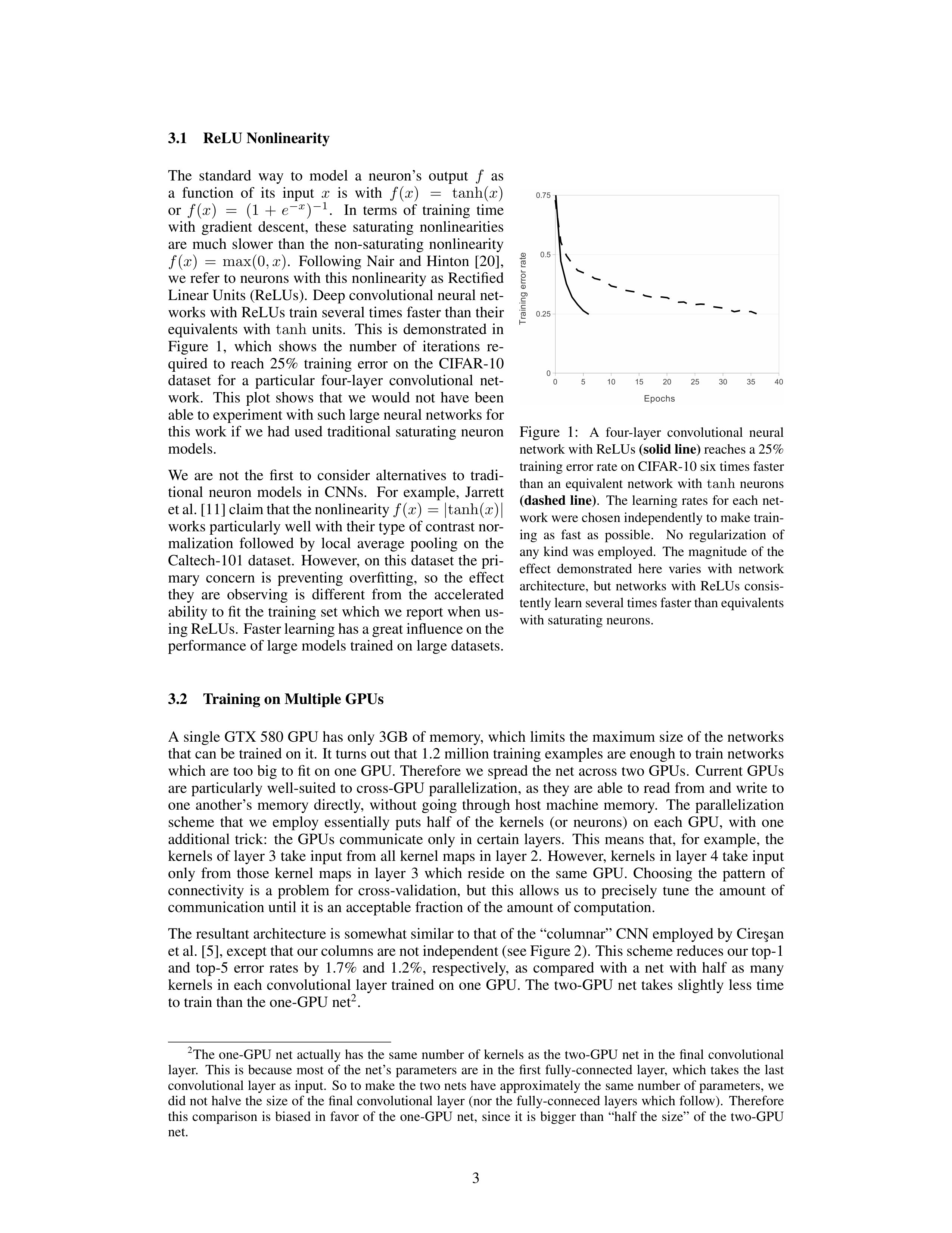
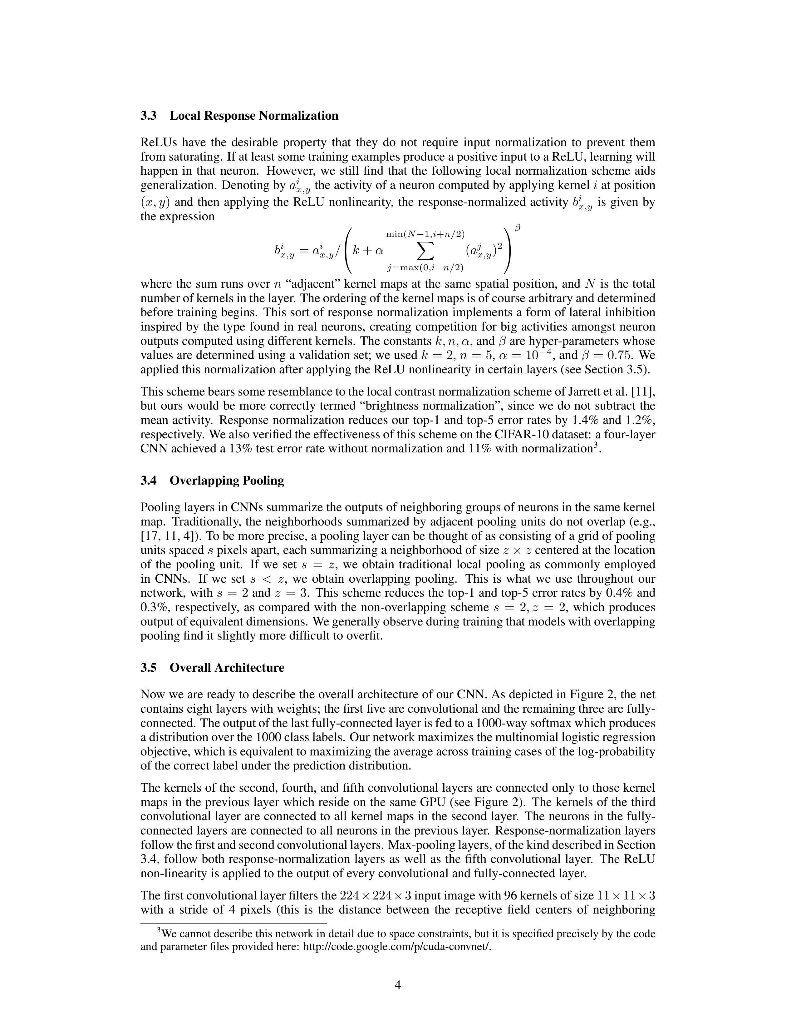
Figure
1:
A
four-layer
convolutional
neural
network with ReLUs
(solid line)
reaches a 25%
training error rate on CIFAR-10 six times faster
than
an
equivalent
network
with
tanh
neurons
(dashed line)
.
The learning rates for each net-
work were chosen independently to make train-
ing
as
fast
as
possible.
No
regularization
of
any kind was employed.
The magnitude of the
effect
demonstrated
here
varies
with
network
architecture,
but
networks
with
ReLUs
consis-
tently learn several times faster than equivalents
with saturating neurons.
The
standard
way
to
model
a
neuron’s
output
f
as
a
function
of
its
input
x
is
with
f
(
x
)
=
tanh(
x
)
or
f
(
x
)
=
(1
+
e
−
x
)
−
1
.
In
terms
of
training
time
with
gradient
descent,
these
saturating
nonlinearities
are
much
slower
than
the
non-saturating
nonlinearity
f
(
x
)
=
max(0
, x
)
.
Following
Nair
and
Hinton
[20],
we refer to neurons with this nonlinearity as Rectified
Linear Units (ReLUs).
Deep convolutional neural net-
works with ReLUs train several times faster than their
equivalents
with
tanh
units.
This
is
demonstrated
in
Figure
1,
which
shows
the
number
of
iterations
re-
quired
to
reach
25%
training
error
on
the
CIFAR-10
dataset
for
a
particular
four-layer
convolutional
net-
work.
This
plot
shows
that
we
would
not
have
been
able to experiment with such large neural networks for
this work if we had used traditional saturating neuron
models.
We
are
not
the
first
to
consider
alternatives
to
tradi-
tional
neuron
models
in
CNNs.
For
example,
Jarrett
et al. [11] claim that the nonlinearity
f
(
x
) =
|
tanh(
x
)
|
works particularly well with their type of contrast nor-
malization
followed
by
local
average
pooling
on
the
Caltech-101 dataset.
However, on this dataset the pri-
mary
concern
is
preventing
overfitting,
so
the
effect
they
are
observing
is
different
from
the
accelerated
ability to fit the training set which we report when us-
ing ReLUs. Faster learning has a great influence on the
performance of large models trained on large datasets.
3.2
Training on Multiple GPUs
A single GTX 580 GPU has only 3GB of memory, which limits the maximum size of the networks
that can be trained on it.
It turns out that 1.2 million training examples are enough to train networks
which are too big to fit on one GPU. Therefore we spread the net across two GPUs.
Current GPUs
are particularly well-suited to cross-GPU parallelization, as they are able to read from and write to
one
another’s
memory
directly,
without
going
through
host
machine
memory.
The
parallelization
scheme
that
we
employ
essentially
puts
half
of
the
kernels
(or
neurons)
on
each
GPU,
with
one
additional
trick:
the
GPUs
communicate
only
in
certain
layers.
This
means
that,
for
example,
the
kernels of layer 3 take input from all kernel maps in layer 2.
However, kernels in layer 4 take input
only
from
those
kernel
maps
in
layer
3
which
reside
on
the
same
GPU.
Choosing
the
pattern
of
connectivity
is
a
problem
for
cross-validation,
but
this
allows
us
to
precisely
tune
the
amount
of
communication until it is an acceptable fraction of the amount of computation.
The resultant architecture is somewhat similar to that of the “columnar” CNN employed by Cire¸san
et al. [5], except that our columns are not independent (see Figure 2). This scheme reduces our top-1
and
top-5
error
rates
by
1.7%
and
1.2%,
respectively,
as
compared
with
a
net
with
half
as
many
kernels in each convolutional layer trained on one GPU. The two-GPU net takes slightly less time
to train than the one-GPU net
2
.
2
The one-GPU net actually has the same number of kernels as the two-GPU net in the final convolutional
layer.
This
is
because
most
of
the
net’s
parameters
are
in
the
first
fully-connected
layer,
which
takes
the
last
convolutional layer as input.
So to make the two nets have approximately the same number of parameters, we
did not halve the size of the final convolutional layer (nor the fully-conneced layers which follow).
Therefore
this
comparison
is
biased
in
favor
of
the
one-GPU
net,
since
it
is
bigger
than
“half
the
size”
of
the
two-GPU
net.
3
3.3
Local Response Normalization
ReLUs
have
the
desirable
property
that
they
do
not
require
input
normalization
to
prevent
them
from saturating.
If at least some training examples produce a positive input to a ReLU, learning will
happen
in
that
neuron.
However,
we
still
find
that
the
following
local
normalization
scheme
aids
generalization.
Denoting by
a
i
x,y
the activity of a neuron computed by applying kernel
i
at position
(
x, y
)
and
then
applying
the
ReLU
nonlinearity,
the
response-normalized
activity
b
i
x,y
is
given
by
the expression
b
i
x,y
=
a
i
x,y
/
k
+
α
min(
N
−
1
,i
+
n/
2)
X
j
=max(0
,i
−
n/
2)
(
a
j
x,y
)
2
β
where
the
sum
runs
over
n
“adjacent” kernel
maps at
the same
spatial position,
and
N
is the
total
number of kernels in the layer. The ordering of the kernel maps is of course arbitrary and determined
before training begins.
This sort of response normalization implements a form of lateral inhibition
inspired
by
the
type
found
in
real
neurons,
creating
competition
for
big
activities
amongst
neuron
outputs computed using different kernels.
The constants
k, n, α
, and
β
are hyper-parameters whose
values are determined using a validation set; we used
k
=
2
,
n
=
5
,
α
=
10
−
4
, and
β
=
0
.
75
.
We
applied this normalization after applying the ReLU nonlinearity in certain layers (see Section 3.5).
This scheme bears some resemblance to the local contrast normalization scheme of Jarrett et al. [11],
but
ours
would
be
more
correctly
termed
“brightness
normalization”,
since
we
do
not
subtract
the
mean activity.
Response normalization reduces our top-1 and top-5 error rates by 1.4% and 1.2%,
respectively.
We also verified the effectiveness of this scheme on the CIFAR-10 dataset: a four-layer
CNN achieved a 13% test error rate without normalization and 11% with normalization
3
.
3.4
Overlapping Pooling
Pooling layers in CNNs summarize the outputs of neighboring groups of neurons in the same kernel
map.
Traditionally,
the neighborhoods summarized by adjacent pooling units do not overlap (e.g.,
[17, 11, 4]).
To be more precise, a pooling layer can be thought of as consisting of a grid of pooling
units spaced
s
pixels apart, each summarizing a neighborhood of size
z
×
z
centered at the location
of
the
pooling
unit.
If
we
set
s
=
z
,
we
obtain
traditional
local
pooling
as
commonly
employed
in
CNNs.
If
we
set
s
<
z
,
we
obtain
overlapping
pooling.
This
is
what
we
use
throughout
our
network, with
s
=
2
and
z
=
3
.
This scheme reduces the top-1 and top-5 error rates by 0.4% and
0.3%,
respectively,
as
compared
with
the
non-overlapping
scheme
s
=
2
, z
=
2
,
which
produces
output of equivalent dimensions. We generally observe during training that models with overlapping
pooling find it slightly more difficult to overfit.
3.5
Overall Architecture
Now we are ready to describe the overall architecture of our CNN. As depicted in Figure 2, the net
contains eight layers with weights; the first five are convolutional and the remaining three are fully-
connected. The output of the last fully-connected layer is fed to a 1000-way softmax which produces
a distribution over the 1000 class labels. Our network maximizes the multinomial logistic regression
objective, which is equivalent to maximizing the average across training cases of the log-probability
of the correct label under the prediction distribution.
The kernels of the second, fourth, and fifth convolutional layers are connected only to those kernel
maps in the previous layer which reside on the same GPU (see Figure 2).
The kernels of the third
convolutional layer are connected to all kernel maps in the second layer.
The neurons in the fully-
connected layers are connected to all neurons in the previous layer.
Response-normalization layers
follow the first and second convolutional layers. Max-pooling layers, of the kind described in Section
3.4,
follow
both
response-normalization
layers
as
well
as
the
fifth
convolutional
layer.
The
ReLU
non-linearity is applied to the output of every convolutional and fully-connected layer.
The first convolutional layer filters the
224
×
224
×
3
input image with 96 kernels of size
11
×
11
×
3
with
a
stride
of
4
pixels
(this
is
the
distance
between
the
receptive
field
centers
of
neighboring
3
We cannot describe this network in detail due to space constraints, but it is specified precisely by the code
and parameter files provided here:
http://code.google.com/p/cuda-convnet/.
4
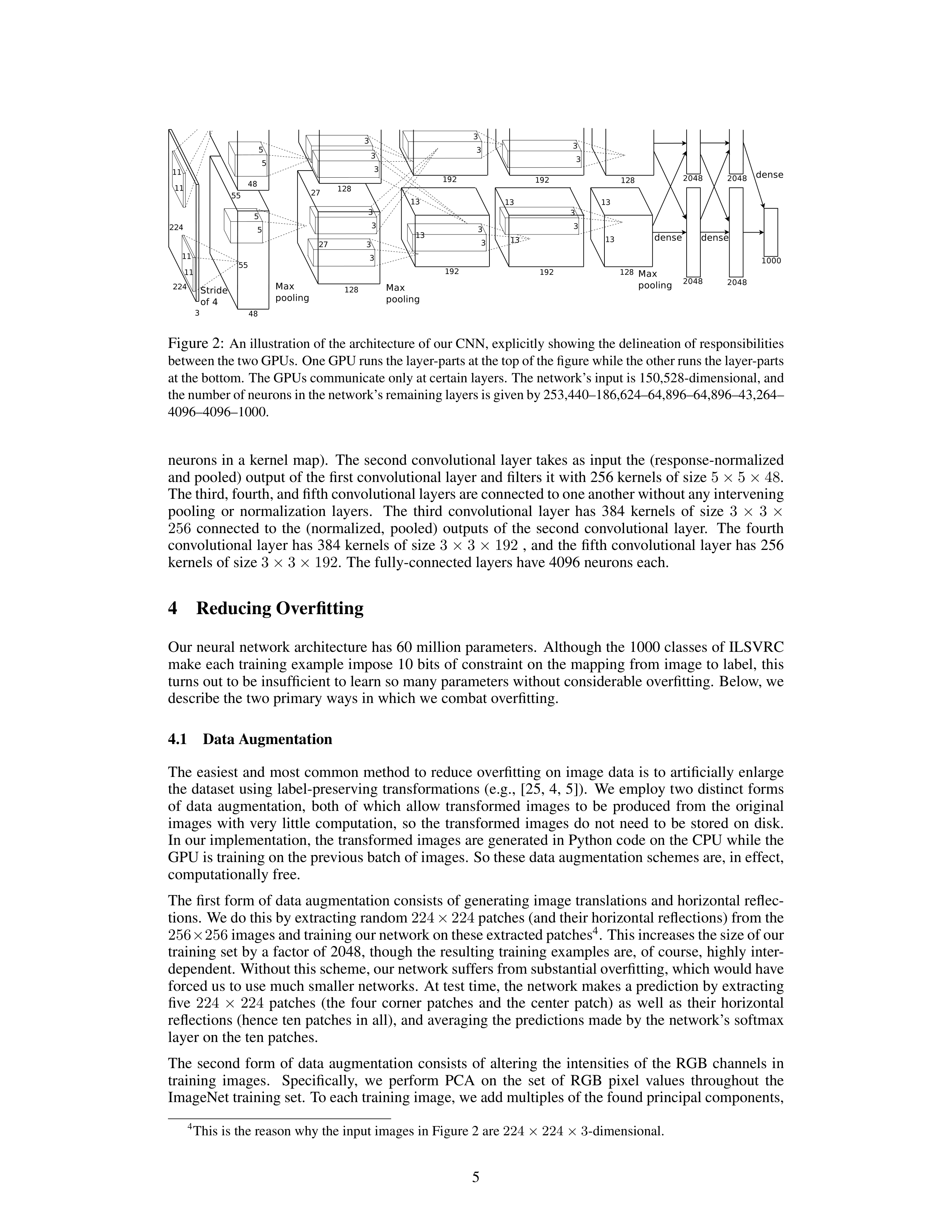
Figure 2:
An illustration of the architecture of our CNN, explicitly showing the delineation of responsibilities
between the two GPUs. One GPU runs the layer-parts at the top of the figure while the other runs the layer-parts
at the bottom.
The GPUs communicate only at certain layers.
The network’s input is 150,528-dimensional, and
the number of neurons in the network’s remaining layers is given by 253,440–186,624–64,896–64,896–43,264–
4096–4096–1000.
neurons in a kernel map).
The second convolutional layer takes as input the (response-normalized
and pooled) output of the first convolutional layer and filters it with 256 kernels of size
5
×
5
×
48
.
The third, fourth, and fifth convolutional layers are connected to one another without any intervening
pooling
or
normalization
layers.
The
third
convolutional
layer
has
384
kernels
of
size
3
×
3
×
256
connected
to
the
(normalized,
pooled)
outputs
of
the
second
convolutional
layer.
The
fourth
convolutional layer has 384 kernels of size
3
×
3
×
192
, and the fifth convolutional layer has 256
kernels of size
3
×
3
×
192
.
The fully-connected layers have 4096 neurons each.
4
Reducing Overfitting
Our neural network architecture has 60 million parameters.
Although the 1000 classes of ILSVRC
make each training example impose 10 bits of constraint on the mapping from image to label, this
turns out to be insufficient to learn so many parameters without considerable overfitting.
Below, we
describe the two primary ways in which we combat overfitting.
4.1
Data Augmentation
The easiest and most common method to reduce overfitting on image data is to artificially enlarge
the dataset using label-preserving transformations (e.g.,
[25, 4, 5]).
We employ two distinct forms
of
data
augmentation,
both
of
which
allow
transformed
images
to
be
produced
from
the
original
images
with
very
little
computation,
so
the
transformed
images
do
not
need
to
be
stored
on
disk.
In our implementation, the transformed images are generated in Python code on the CPU while the
GPU is training on the previous batch of images.
So these data augmentation schemes are, in effect,
computationally free.
The first form of data augmentation consists of generating image translations and horizontal reflec-
tions.
We do this by extracting random
224
×
224
patches (and their horizontal reflections) from the
256
×
256
images and training our network on these extracted patches
4
. This increases the size of our
training set by a factor of 2048, though the resulting training examples are, of course, highly inter-
dependent.
Without this scheme, our network suffers from substantial overfitting, which would have
forced us to use much smaller networks.
At test time, the network makes a prediction by extracting
five
224
×
224
patches
(the
four
corner
patches
and
the
center
patch)
as
well
as
their
horizontal
reflections (hence ten patches in all), and averaging the predictions made by the network’s softmax
layer on the ten patches.
The
second
form
of
data
augmentation
consists
of
altering
the
intensities
of
the
RGB
channels
in
training
images.
Specifically,
we
perform
PCA
on
the
set
of
RGB
pixel
values
throughout
the
ImageNet training set.
To each training image, we add multiples of the found principal components,
4
This is the reason why the input images in Figure 2 are
224
×
224
×
3
-dimensional.
5
with magnitudes proportional to the corresponding eigenvalues times a random variable drawn from
a Gaussian with mean zero and standard deviation 0.1.
Therefore to each RGB image pixel
I
xy
=
[
I
R
xy
, I
G
xy
, I
B
xy
]
T
we add the following quantity:
[
p
1
,
p
2
,
p
3
][
α
1
λ
1
, α
2
λ
2
, α
3
λ
3
]
T
where
p
i
and
λ
i
are
i
th
eigenvector
and
eigenvalue
of
the
3
×
3
covariance
matrix
of
RGB
pixel
values,
respectively,
and
α
i
is
the
aforementioned
random
variable.
Each
α
i
is
drawn
only
once
for all the pixels of a particular training image until that image is used for training again, at which
point it is re-drawn.
This scheme approximately captures an important property of natural images,
namely, that object identity is invariant to changes in the intensity and color of the illumination. This
scheme reduces the top-1 error rate by over 1%.
4.2
Dropout
Combining the predictions of many different models is a very successful way to reduce test errors
[1,
3],
but
it
appears
to
be
too
expensive
for
big
neural
networks
that
already
take
several
days
to
train.
There
is,
however,
a
very
efficient
version
of
model
combination
that
only
costs
about
a
factor
of
two
during
training.
The
recently-introduced
technique,
called
“dropout”
[10],
consists
of
setting
to
zero
the
output
of
each
hidden
neuron
with
probability
0.5.
The
neurons
which
are
“dropped
out”
in
this
way
do
not
contribute
to
the
forward
pass
and
do
not
participate
in
back-
propagation. So every time an input is presented, the neural network samples a different architecture,
but all these architectures share weights. This technique reduces complex co-adaptations of neurons,
since
a
neuron
cannot
rely
on
the
presence
of
particular
other
neurons.
It
is,
therefore,
forced
to
learn more robust features that are useful in conjunction with many different random subsets of the
other
neurons.
At
test
time,
we
use
all
the
neurons
but
multiply
their
outputs
by
0.5,
which
is
a
reasonable approximation to taking the geometric mean of the predictive distributions produced by
the exponentially-many dropout networks.
We use dropout in the first two fully-connected layers of Figure 2. Without dropout, our network ex-
hibits substantial overfitting. Dropout roughly doubles the number of iterations required to converge.
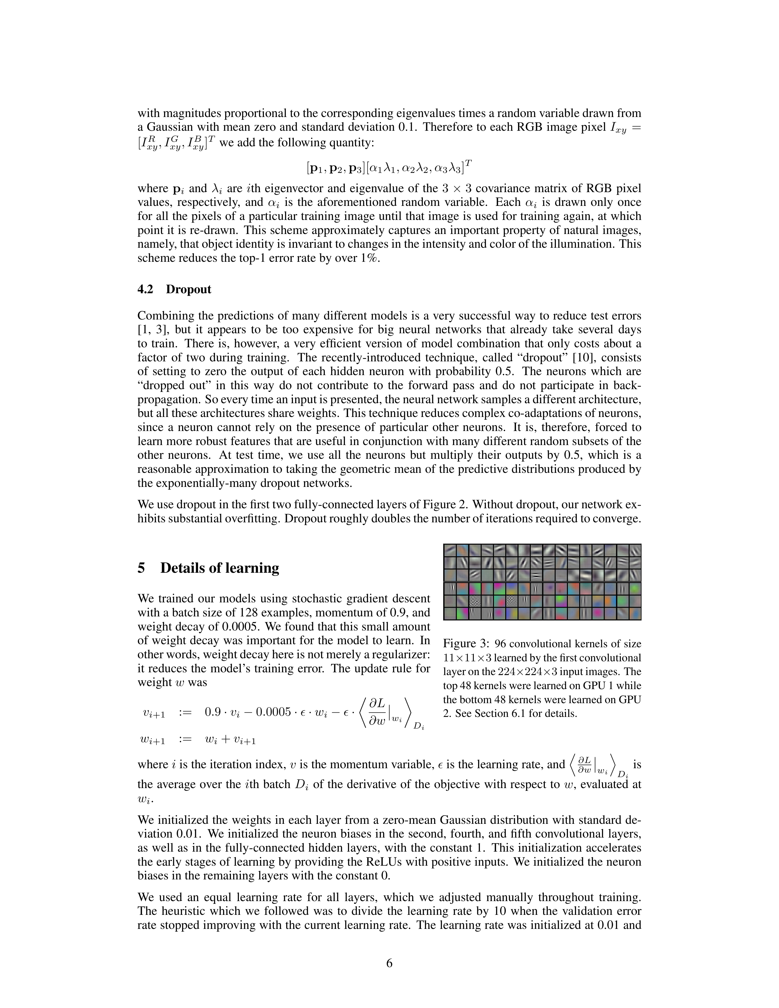
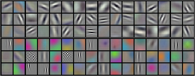
Figure 3:
96 convolutional kernels of size
11
×
11
×
3
learned by the first convolutional
layer on the
224
×
224
×
3
input images. The
top 48 kernels were learned on GPU 1 while
the bottom 48 kernels were learned on GPU
2.
See Section 6.1 for details.
5
Details of learning
We
trained
our
models
using
stochastic
gradient
descent
with a batch size of 128 examples, momentum of 0.9, and
weight decay of 0.0005.
We found that this small amount
of weight decay was important for the model to learn.
In
other words, weight decay here is not merely a regularizer:
it
reduces
the
model’s
training
error.
The
update
rule
for
weight
w
was
v
i
+1
:=
0
.
9
·
v
i
−
0
.
0005
·
ϵ
·
w
i
−
ϵ
·
∂L
∂w
w
i
D
i
w
i
+1
:=
w
i
+
v
i
+1
where
i
is the iteration index,
v
is the momentum variable,
ϵ
is the learning rate, and
D
∂L
∂w
w
i
E
D
i
is
the
average
over
the
i
th
batch
D
i
of
the
derivative
of
the
objective
with
respect
to
w
,
evaluated
at
w
i
.
We initialized
the
weights in each
layer from a zero-mean Gaussian distribution with standard de-
viation 0.01.
We initialized the neuron biases in the second,
fourth,
and fifth convolutional layers,
as
well
as
in
the
fully-connected
hidden
layers,
with
the
constant
1.
This
initialization
accelerates
the early stages of learning by providing the ReLUs with positive inputs.
We initialized the neuron
biases in the remaining layers with the constant 0.
We
used
an
equal
learning
rate
for
all
layers,
which
we
adjusted
manually
throughout
training.
The
heuristic
which
we
followed
was
to
divide
the
learning
rate
by
10
when
the
validation
error
rate stopped improving with the current learning rate.
The learning rate was initialized at 0.01 and
6
reduced three times prior to termination.
We trained the network for roughly 90 cycles through the
training set of 1.2 million images, which took five to six days on two NVIDIA GTX 580 3GB GPUs.
6
Results
Our
results
on
ILSVRC-2010
are
summarized
in
Table
1.
Our
network
achieves
top-1
and
top-5
test
set
error
rates
of
37.5%
and
17.0%
5
.
The
best
performance
achieved
during
the
ILSVRC-
2010
competition
was
47.1%
and
28.2%
with
an
approach
that
averages
the
predictions
produced
from
six
sparse-coding
models
trained
on
different
features
[2],
and
since
then
the
best
pub-
lished
results
are
45.7%
and
25.7%
with
an
approach
that
averages
the
predictions
of
two
classi-
fiers
trained
on
Fisher
Vectors
(FVs)
computed
from
two
types
of
densely-sampled
features
[24].
Model
Top-1
Top-5
Sparse coding [2]
47.1%
28.2%
SIFT + FVs [24]
45.7%
25.7%
CNN
37.5%
17.0%
Table 1:
Comparison of results on ILSVRC-
2010
test
set.
In
italics
are
best
results
achieved by others.
We
also
entered
our
model
in
the
ILSVRC-2012
com-
petition
and
report
our
results
in
Table
2.
Since
the
ILSVRC-2012
test
set
labels
are
not
publicly
available,
we
cannot
report
test
error
rates
for
all
the
models
that
we
tried.
In
the
remainder
of
this
paragraph,
we
use
validation
and
test
error
rates
interchangeably
because
in our experience they do not differ by more than 0.1%
(see Table 2).
The CNN described in this paper achieves
a
top-5
error
rate
of
18.2%.
Averaging
the
predictions
of
five
similar
CNNs
gives
an
error
rate
of
16.4%.
Training
one
CNN,
with
an
extra
sixth
con-
volutional
layer
over
the
last
pooling
layer,
to
classify
the
entire
ImageNet
Fall
2011
release
(15M
images,
22K
categories),
and
then
“fine-tuning”
it
on
ILSVRC-2012
gives
an
error
rate
of
16.6%.
Averaging
the
predictions
of
two
CNNs
that
were
pre-trained
on
the
entire
Fall
2011
re-
lease
with
the
aforementioned
five
CNNs
gives
an
error
rate
of
15.3%
.
The
second-best
con-
test
entry
achieved
an
error
rate
of
26.2%
with
an
approach
that
averages
the
predictions
of
sev-
eral
classifiers
trained
on
FVs
computed
from
different
types
of
densely-sampled
features
[7].
Model
Top-1 (val)
Top-5 (val)
Top-5 (test)
SIFT + FVs [7]
—
—
26.2%
1 CNN
40.7%
18.2%
—
5 CNNs
38.1%
16.4%
16.4%
1 CNN*
39.0%
16.6%
—
7 CNNs*
36.7%
15.4%
15.3%
Table
2:
Comparison
of
error
rates
on
ILSVRC-2012
validation
and
test sets.
In
italics
are best results achieved by others.
Models with an
asterisk* were “pre-trained” to classify the entire ImageNet 2011 Fall
release.
See Section 6 for details.
Finally,
we
also
report
our
error
rates
on
the
Fall
2009
version
of
ImageNet with 10,184 categories
and
8.9
million
images.
On
this
dataset we follow the convention
in
the
literature
of
using
half
of
the
images
for
training
and
half
for
testing.
Since
there
is
no
es-
tablished test set, our split neces-
sarily differs from the splits used
by previous authors, but this does
not affect the results appreciably.
Our
top-1
and
top-5
error
rates
on
this
dataset
are
67.4%
and
40.9%
, attained by the net described above but with an additional, sixth convolutional layer over the
last pooling layer.
The best published results on this dataset are 78.1% and 60.9% [19].
6.1
Qualitative Evaluations
Figure 3 shows the convolutional kernels learned by the network’s two data-connected layers.
The
network has learned a variety of frequency- and orientation-selective kernels, as well as various col-
ored blobs.
Notice the specialization exhibited by the two GPUs, a result of the restricted connec-
tivity described in Section 3.5.
The kernels on GPU 1 are largely color-agnostic, while the kernels
on on GPU 2 are largely color-specific.
This kind of specialization occurs during every run and is
independent of any particular random weight initialization (modulo a renumbering of the GPUs).
5
The error rates without averaging predictions over ten patches as described in Section 4.1 are 39.0% and
18.3%.
7
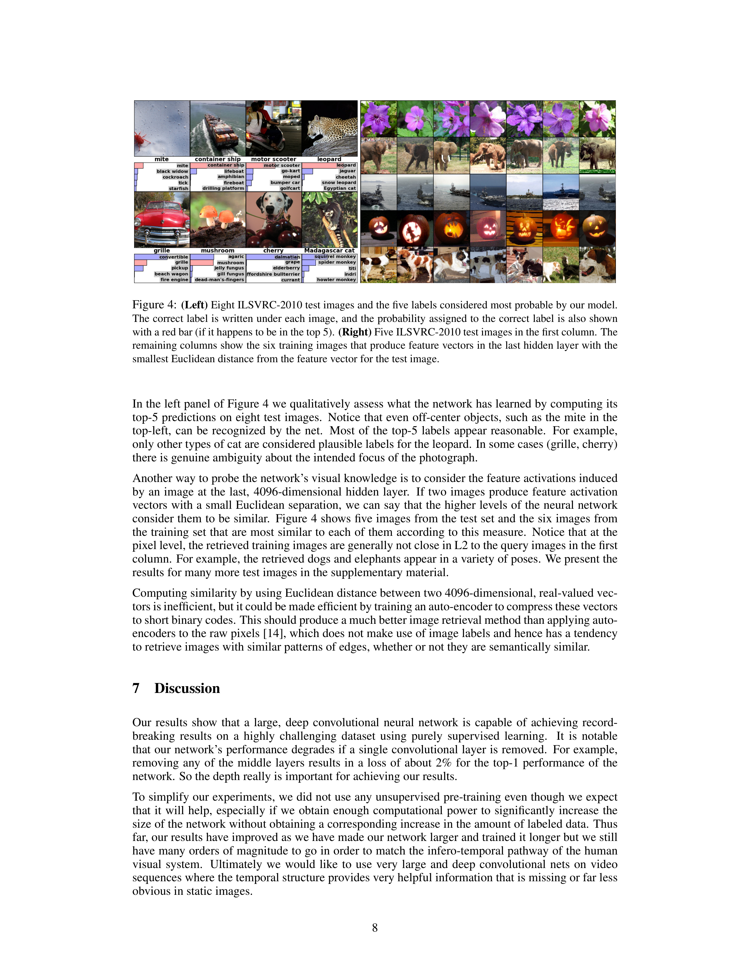
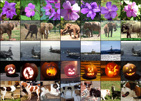
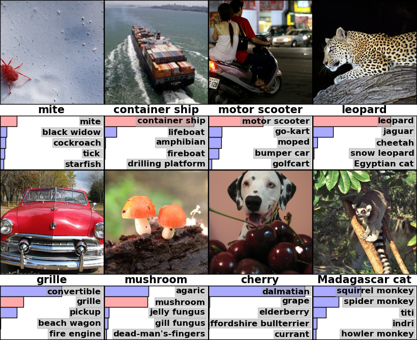
Figure 4:
(Left)
Eight ILSVRC-2010 test images and the five labels considered most probable by our model.
The
correct
label
is
written
under
each
image,
and
the
probability
assigned
to
the
correct
label
is
also
shown
with a red bar (if it happens to be in the top 5).
(Right)
Five ILSVRC-2010 test images in the first column.
The
remaining columns show the six training images that produce feature vectors in the last hidden layer with the
smallest Euclidean distance from the feature vector for the test image.
In the left panel of Figure 4 we qualitatively assess what the network has learned by computing its
top-5
predictions
on
eight
test
images.
Notice
that
even
off-center
objects,
such
as
the
mite
in
the
top-left,
can
be
recognized
by
the
net.
Most
of
the
top-5
labels
appear
reasonable.
For
example,
only other types of cat are considered plausible labels for the leopard.
In some cases (grille, cherry)
there is genuine ambiguity about the intended focus of the photograph.
Another way to probe the network’s visual knowledge is to consider the feature activations induced
by
an
image
at
the
last,
4096-dimensional
hidden
layer.
If
two
images
produce
feature
activation
vectors
with
a
small
Euclidean
separation,
we
can
say
that
the
higher
levels
of
the
neural
network
consider them to be similar.
Figure 4 shows five images from the test set and the six images from
the training
set
that
are
most
similar to each of them according to this measure.
Notice that at the
pixel level, the retrieved training images are generally not close in L2 to the query images in the first
column.
For example, the retrieved dogs and elephants appear in a variety of poses.
We present the
results for many more test images in the supplementary material.
Computing similarity by using Euclidean distance between two 4096-dimensional, real-valued vec-
tors is inefficient, but it could be made efficient by training an auto-encoder to compress these vectors
to short binary codes. This should produce a much better image retrieval method than applying auto-
encoders to the raw pixels [14], which does not make use of image labels and hence has a tendency
to retrieve images with similar patterns of edges, whether or not they are semantically similar.
7
Discussion
Our
results
show
that
a
large,
deep
convolutional
neural
network
is
capable
of
achieving
record-
breaking
results
on
a
highly
challenging
dataset
using
purely
supervised
learning.
It
is
notable
that
our
network’s
performance
degrades
if
a
single
convolutional
layer
is
removed.
For
example,
removing
any
of
the
middle
layers
results
in
a
loss
of
about
2%
for
the
top-1
performance
of
the
network.
So the depth really is important for achieving our results.
To simplify our experiments, we did not use any unsupervised pre-training even though we expect
that
it
will
help,
especially
if
we
obtain
enough
computational
power
to
significantly
increase
the
size of the network without obtaining a corresponding increase in the amount of labeled data.
Thus
far, our results have improved as we have made our network larger and trained it longer but we still
have many orders of magnitude to go in order to match the infero-temporal pathway of the human
visual
system.
Ultimately
we
would
like
to
use
very
large
and
deep
convolutional
nets
on
video
sequences where the temporal structure provides very helpful information that is missing or far less
obvious in static images.
8
References
[1]
R.M. Bell and Y. Koren. Lessons from the netflix prize challenge.
ACM SIGKDD Explorations Newsletter
,
9(2):75–79, 2007.
[2]
A.
Berg,
J.
Deng,
and
L.
Fei-Fei.
Large
scale
visual
recognition
challenge
2010.
www.image-
net.org/challenges.
2010.
[3]
L. Breiman.
Random forests.
Machine learning
, 45(1):5–32, 2001.
[4]
D. Cire¸san, U. Meier, and J. Schmidhuber.
Multi-column deep neural networks for image classification.
Arxiv preprint arXiv:1202.2745
, 2012.
[5]
D.C.
Cire¸san,
U.
Meier,
J.
Masci,
L.M.
Gambardella,
and
J.
Schmidhuber.
High-performance
neural
networks for visual object classification.
Arxiv preprint arXiv:1102.0183
, 2011.
[6]
J.
Deng,
W.
Dong,
R.
Socher,
L.-J.
Li,
K.
Li,
and
L.
Fei-Fei.
ImageNet:
A
Large-Scale
Hierarchical
Image Database.
In
CVPR09
, 2009.
[7]
J.
Deng,
A.
Berg,
S.
Satheesh,
H.
Su,
A.
Khosla,
and
L.
Fei-Fei.
ILSVRC-2012
,
2012.
URL
http://www.image-net.org/challenges/LSVRC/2012/
.
[8]
L. Fei-Fei, R. Fergus, and P. Perona.
Learning generative visual models from few training examples:
An
incremental bayesian approach tested on 101 object categories.
Computer Vision and Image Understand-
ing
, 106(1):59–70, 2007.
[9]
G. Griffin,
A. Holub,
and P. Perona.
Caltech-256 object category dataset.
Technical Report 7694,
Cali-
fornia Institute of Technology, 2007.
URL
http://authors.library.caltech.edu/7694
.
[10]
G.E. Hinton, N. Srivastava, A. Krizhevsky, I. Sutskever, and R.R. Salakhutdinov.
Improving neural net-
works by preventing co-adaptation of feature detectors.
arXiv preprint arXiv:1207.0580
, 2012.
[11]
K. Jarrett, K. Kavukcuoglu, M. A. Ranzato, and Y. LeCun.
What is the best multi-stage architecture for
object recognition?
In
International Conference on Computer Vision
, pages 2146–2153. IEEE, 2009.
[12]
A.
Krizhevsky.
Learning
multiple
layers
of
features
from
tiny
images.
Master’s
thesis,
Department
of
Computer Science, University of Toronto, 2009.
[13]
A. Krizhevsky.
Convolutional deep belief networks on cifar-10.
Unpublished manuscript
, 2010.
[14]
A.
Krizhevsky
and
G.E.
Hinton.
Using
very
deep
autoencoders
for
content-based
image
retrieval.
In
ESANN
, 2011.
[15]
Y.
Le
Cun,
B.
Boser,
J.S.
Denker,
D.
Henderson,
R.E.
Howard,
W.
Hubbard,
L.D.
Jackel,
et
al.
Hand-
written digit recognition with a back-propagation network.
In
Advances in neural information processing
systems
, 1990.
[16]
Y. LeCun, F.J. Huang, and L. Bottou.
Learning methods for generic object recognition with invariance to
pose
and
lighting.
In
Computer
Vision
and
Pattern
Recognition,
2004.
CVPR
2004.
Proceedings
of
the
2004 IEEE Computer Society Conference on
, volume 2, pages II–97. IEEE, 2004.
[17]
Y.
LeCun,
K.
Kavukcuoglu,
and
C.
Farabet.
Convolutional
networks
and
applications
in
vision.
In
Circuits and Systems (ISCAS), Proceedings of 2010 IEEE International Symposium on
,
pages 253–256.
IEEE, 2010.
[18]
H. Lee, R. Grosse, R. Ranganath, and A.Y. Ng.
Convolutional deep belief networks for scalable unsuper-
vised learning of hierarchical representations. In
Proceedings of the 26th Annual International Conference
on Machine Learning
, pages 609–616. ACM, 2009.
[19]
T.
Mensink,
J.
Verbeek,
F.
Perronnin,
and
G.
Csurka.
Metric
Learning
for
Large
Scale
Image
Classifi-
cation:
Generalizing to New Classes at Near-Zero Cost.
In
ECCV - European Conference on Computer
Vision
, Florence, Italy, October 2012.
[20]
V.
Nair
and
G.
E.
Hinton.
Rectified
linear
units
improve
restricted
boltzmann
machines.
In
Proc.
27th
International Conference on Machine Learning
, 2010.
[21]
N. Pinto, D.D. Cox, and J.J. DiCarlo.
Why is real-world visual object recognition hard?
PLoS computa-
tional biology
, 4(1):e27, 2008.
[22]
N. Pinto, D. Doukhan, J.J. DiCarlo, and D.D. Cox.
A high-throughput screening approach to discovering
good forms of biologically inspired visual representation.
PLoS computational biology
, 5(11):e1000579,
2009.
[23]
B.C. Russell, A. Torralba, K.P. Murphy, and W.T. Freeman.
Labelme:
a database and web-based tool for
image annotation.
International journal of computer vision
, 77(1):157–173, 2008.
[24]
J. Sánchez and F. Perronnin. High-dimensional signature compression for large-scale image classification.
In
Computer Vision and Pattern Recognition (CVPR), 2011 IEEE Conference on
, pages 1665–1672. IEEE,
2011.
[25]
P.Y.
Simard,
D.
Steinkraus,
and
J.C.
Platt.
Best
practices
for
convolutional
neural
networks
applied
to
visual document analysis.
In
Proceedings of the Seventh International Conference on Document Analysis
and Recognition
, volume 2, pages 958–962, 2003.
[26]
S.C. Turaga, J.F. Murray, V. Jain, F. Roth, M. Helmstaedter, K. Briggman, W. Denk, and H.S. Seung. Con-
volutional networks can learn to generate affinity graphs for image segmentation.
Neural Computation
,
22(2):511–538, 2010.
9